Documentation of Handbook Model

View the 180 variables sorted by type, module, variable name, module/group/name, view, or in a view summary.

Model Assessment Results

Description	Number
Equations with Embedded Data	32
Incompletely Defined Variables	0
Overly Complex Stock Formulation	0
Overly Complex Formulation (Richardson's Rule = 3)	16
Undocumented Equations	1
Unused Variables	3
Variables Not in Any View	0



Supplementary Variables	8
Supplementary Variables Being Used	0
Warnings	2

Types:

S : Stock (11)	SM : Smooth (6)	SI : Stock Initial (10)	I : Initial (5)	L : Lookup (8)
C : Constant (78)	F : Flow (16)	A : Auxiliary (72)	Sub: Subscripts (0)	D : Data (0)
G : Game (0)

Groups:

Control (4) Simulation Control Parameters	Individual Learning Curve (4) Display of Average Learning Curve	Market Response (19) Service Attractiveness and Market Size	Normalized Responses (6) Display of Fractional Responses to Work Pressure	Service Quality (10) Error Generation and Perceived Quality
Task Flows (15) Backlog, Rework and Balking	Test Generator for Absenteeism (19)	Test Generator for Arrivals (20)	Test Switches (6) Structure Control Switches	Time per Task (10) Adjustments to Time per Task
Workforce (37) Employee Hiring, Training, and Turnover	Workforce Planning (18) Workforce Requirements and Authorization	Workweek (12) Adjustments to Workweek

Modules:

Default (180)

Views:

Workforce (41)	Effective, Desired and Authorized Workforce (34)	Backlog (45)	Standard Time per Task (7)	Service Quailty (17)
Task Arrivals and Absenteeism (49)	Responses (14)	Market Response (26)	Not Present In Any View (0)

TOP	Control
Module	*Group*	Type	Variable Name and Description
Default	Control	C	FINAL TIME (Week) = 250 Description: The final time for the simulation. Not Present In Any View
Default	Control	C	INITIAL TIME (Week) = 0 Description: The initial time for the simulation. Not Present In Any View Used by: Time - Internally defined simulation time.
Default	Control	C	SAVEPER (Week [0,?]) = 0.125 Description: The frequency with which output is stored. Not Present In Any View
Default	Control	C	TIME STEP (Week [0,?]) = 0.0078125 Description: The time step for the simulation. Present in 1 view: Task Arrivals and Absenteeism Used by: White Noise 0 - White noise input to the pink noise process. White Noise - White noise input to the pink noise process.
TOP	Individual Learning Curve
Module	*Group*	Type	Variable Name and Description
Default	Individual Learning Curve	A	LC (Employees) = LC E+LC RRookie productivity fraction Description:* Average individual learning curve. Created exclusively for reporting purposes. Estimates the individual learning curve by reporting the productivity of a single individual as it makes the transition from rookie to experienced employee. Formulation is equivalent to workforce productivity, but limited to a single employee and with no effects from hiring and turnover rates, Present in 1 view: Effective, Desired and Authorized Workforce Used by: This is a supplementary variable.
Default	Individual Learning Curve	F,A	LC AR (Employees/Week) = LC R/Assimilation Time Description: Assimilation rate for the individual learning curve. Present in 1 view: Effective, Desired and Authorized Workforce Used by: LC E - Experienced employee for the estimation of the individual learning curve. Initialized at zero to reflect the fact that an initial employee has no experience. LC R - Rookie employee for the estimation of the individual learning curve. Initialized at one to reflect the fact that at time zero an employee has no experience.
Default	Individual Learning Curve	S	LC E (Employees) = ∫ (LC AR) dt + [0] Description: Experienced employee for the estimation of the individual learning curve. Initialized at zero to reflect the fact that an initial employee has no experience. Present in 1 view: Effective, Desired and Authorized Workforce Used by: LC - Average individual learning curve. Created exclusively for reporting purposes. Estimates the individual learning curve by reporting the productivity of a single individual as it makes the transition from rookie to experienced employee. Formulation is equivalent to workforce productivity, but limited to a single employee and with no effects from hiring and turnover rates,
Default	Individual Learning Curve	S	LC R (Employees) = ∫ (-LC AR) dt + [1] Description: Rookie employee for the estimation of the individual learning curve. Initialized at one to reflect the fact that at time zero an employee has no experience. Present in 1 view: Effective, Desired and Authorized Workforce Used by: LC - Average individual learning curve. Created exclusively for reporting purposes. Estimates the individual learning curve by reporting the productivity of a single individual as it makes the transition from rookie to experienced employee. Formulation is equivalent to workforce productivity, but limited to a single employee and with no effects from hiring and turnover rates, LC AR - Assimilation rate for the individual learning curve.
TOP	Market Response
Module	*Group*	Type	Variable Name and Description
Default	Market Response	C	Base Customer Growth Rate (1/Week) = 0 Description: Fractional growth rate for customer base; independent of service attractiveness. Could be used to reflect demographic trends. Present in 1 view: Market Response Used by: Net Change to Customer Base - The change on the customer base is a function of the attractiveness of the service and a base growth rate that could respond to demographic trends.
Default	Market Response	A	Base Task Arrival Rate (Task/Week) = Customer BaseTask Request per Customer Description:* Number of task generated by the customer base per week. This base number is latter affected by random factors or test inputs. Present in 1 view: Market Response Used by: Endogenous Task Arrival Rate - Note that the impact of the input on the endogenous task arrival rate would be equivalent to modifying the task request per customer since the base line would be affected by changes in the customer base.
Default	Market Response	S	Customer Base (Customers) = ∫ (Net Change to Customer Base) dt + [Standard Completion Rate/Task Request per Customer] Description: Size of the market for the service setting. Present in 2 views: Effective, Desired and Authorized Workforce Market Response Used by: Net Change to Customer Base - The change on the customer base is a function of the attractiveness of the service and a base growth rate that could respond to demographic trends. Base Task Arrival Rate - Number of task generated by the customer base per week. This base number is latter affected by random factors or test inputs. Revenue - Revenue generated from customer. This is driven by the number of customers in the customer base and not by the number of tasks they generate, thus assuming that customers pay a standard fee regardless of usage.
Default	Market Response	A	Effect of Balking on Attractiveness (Dimensionless) = (1+Effect of Delivery Delay on Balking)^Sensitivity of Attractiveness to Balking Description: This effect is formulated differently from the other three since the input is already a dimensionless fractional deviation from the desired standard (0). The formulation introduces an acceptable unit error. Present in 1 view: Market Response Used by: Service Attractiveness - Service Attractiveness is the multiplicative effect of the effects of balking, delivered quality delivery delay and errors. It changes smoothly over time (see documentation of time to react to service attractiveness.
Default	Market Response	A	Effect of Delivered Quality on Attractiveness (Dimensionless) = (Delivered Quality/Target Delivered Quality)^Sensitivity of Attractiveness to Delivered Quality Description: The deviation from the target delivered quality is adjusted by an exponent that reflects how sensitive customers are to these deviation. Present in 1 view: Market Response Used by: Service Attractiveness - Service Attractiveness is the multiplicative effect of the effects of balking, delivered quality delivery delay and errors. It changes smoothly over time (see documentation of time to react to service attractiveness.
Default	Market Response	A	Effect of Delivery Delay on Attractiveness (Dimensionless) = (Delivery Delay/Target Delivery Delay)^Sensitivity of Attractiveness to Delivery Delay Description: The deviation from the target delivery delay is adjusted by an exponent that reflects how sensitive customers are to these deviations. Present in 1 view: Market Response Used by: Service Attractiveness - Service Attractiveness is the multiplicative effect of the effects of balking, delivered quality delivery delay and errors. It changes smoothly over time (see documentation of time to react to service attractiveness.
Default	Market Response	A	Effect of Errors on Attractiveness (Dimensionless) = (1+Error Discovery Rate/Task Completion Rate)^Sensitivity of Attractiveness to Errors Description: Targeted error discovery rate is zero. The departure from that goal is relative to the total number of tasks being processed. Present in 1 view: Market Response Used by: Service Attractiveness - Service Attractiveness is the multiplicative effect of the effects of balking, delivered quality delivery delay and errors. It changes smoothly over time (see documentation of time to react to service attractiveness.
Default	Market Response	A	Endogenous Task Arrival Rate (Tasks/Week) = Base Task Arrival RateInput Description:* Note that the impact of the input on the endogenous task arrival rate would be equivalent to modifying the task request per customer since the base line would be affected by changes in the customer base. Present in 2 views: Backlog Market Response Used by: Task Arrival Rate - Task Arrivals are set to an exogenous rate. If the market feed back option is active, then the tasks arrival rate depends on the customer base.
Default	Market Response	F,A	Net Change to Customer Base (Customers/Week) = Base Customer Growth RateCustomer Base+(Customer BaseService Attractiveness-Customer Base)/Time for Customer Base to Change Description: The change on the customer base is a function of the attractiveness of the service and a base growth rate that could respond to demographic trends. Present in 1 view: Market Response Used by: Customer Base - Size of the market for the service setting.
Default	Market Response	C	Sensitivity of Attractiveness to Balking (Dimensionless [-6,1]) = -1 Description: Exponent to the effect of balking on service attractiveness. The negative sign indicates that this is inversely coded, i.e., attractiveness drops as balking increases. Present in 1 view: Market Response Used by: Effect of Balking on Attractiveness - This effect is formulated differently from the other three since the input is already a dimensionless fractional deviation from the desired standard (0). The formulation introduces an acceptable unit error.
Default	Market Response	C	Sensitivity of Attractiveness to Delivered Quality (Dimensionless [0,6]) = 0.9 Description: Exponent to the effect of delivery quality on service attractiveness. Present in 1 view: Market Response Used by: Effect of Delivered Quality on Attractiveness - The deviation from the target delivered quality is adjusted by an exponent that reflects how sensitive customers are to these deviation.
Default	Market Response	C	Sensitivity of Attractiveness to Delivery Delay (Dimensionless [-6,1]) = -0.3 Description: Exponent to the effect of delivery delay on service attractiveness. The negative sign indicates that this is inversely coded, i.e., attractiveness drops as delivery delay increase. Present in 1 view: Market Response Used by: Effect of Delivery Delay on Attractiveness - The deviation from the target delivery delay is adjusted by an exponent that reflects how sensitive customers are to these deviations.
Default	Market Response	C	Sensitivity of Attractiveness to Errors (Dimensionless) = -1 Description: Exponent to the effect of errors on service attractiveness. The negative sign indicates that this is inversely coded, i.e., attractiveness drops as errors increase. Present in 1 view: Market Response Used by: Effect of Errors on Attractiveness - Targeted error discovery rate is zero. The departure from that goal is relative to the total number of tasks being processed.
Default	Market Response	SM	Service Attractiveness (Dimensionless) = SMOOTH(Effect of Balking on AttractivenessEffect of Delivered Quality on AttractivenessEffect of Delivery Delay on AttractivenessEffect of Errors on Attractiveness,Time to React to Service Attractiveness) Description:* Service Attractiveness is the multiplicative effect of the effects of balking, delivered quality delivery delay and errors. It changes smoothly over time (see documentation of time to react to service attractiveness. Present in 1 view: Market Response Used by: Net Change to Customer Base - The change on the customer base is a function of the attractiveness of the service and a base growth rate that could respond to demographic trends.
Default	Market Response	SI,A	Standard Completion Rate (Tasks/Week) = Service CapacityStandard Workweek/Standard Time per Task Description:* The standard completion rate is the rate at which tasks would be completed by the current workforce at the standard workday and spending the standard time on each task. Used to initialize the market sector in equilibrium. Present in 2 views: Task Arrivals and Absenteeism Market Response Used by: Customer Base - Size of the market for the service setting. Initial Arrival Rate - The initial rate at which work arrives is set to the initial value of the standard completion rate. Note that the equation type is INITIAL, which ensures that the initial arrival rate remains constant even if the standard completion rate varies. By setting the initial arrival rate to the standard completion rate we ensure that tasks arrive at exactly the rate the organization can handle given the initial staff and standard values for the workday and time per task.
Default	Market Response	C	Target Delivered Quality (Dimensionless) = 1 Description: Target delivered quality is set to one to capture the notion that we need to match the Customer Expected Time per Order. The perception of quality is not a direct reflection of the time allocated since the performance gap (measured in time) goes through the quality table function with the flat tolerance zone. Present in 1 view: Market Response Used by: Effect of Delivered Quality on Attractiveness - The deviation from the target delivered quality is adjusted by an exponent that reflects how sensitive customers are to these deviation.
Default	Market Response	SI,C	Task Request per Customer (Tasks/Week/Customer) = 1 Description: Baseline number of tasks generated by customer per week. Present in 1 view: Market Response Used by: Base Task Arrival Rate - Number of task generated by the customer base per week. This base number is latter affected by random factors or test inputs. Customer Base - Size of the market for the service setting.
Default	Market Response	C	Time for Customer Base to Change (Week) = 4 Description: How long it takes customers to act on their perception of service attractiveness Present in 1 view: Market Response Used by: Net Change to Customer Base - The change on the customer base is a function of the attractiveness of the service and a base growth rate that could respond to demographic trends.
Default	Market Response	C	Time to React to Service Attractiveness (Weeks) = 26 Description: Time constant to adjust the speed of adjustment of service attractiveness. Set to be longer than the time to perceive delivery delay and balking, since service quality is fuzzier and it takes longer to gather enough evidence that things are not as they were. In turn time to perceive delivery delay will be longer than the time to perceive balking, since balking is a more salient event. Present in 1 view: Market Response Used by: Service Attractiveness - Service Attractiveness is the multiplicative effect of the effects of balking, delivered quality delivery delay and errors. It changes smoothly over time (see documentation of time to react to service attractiveness.
TOP	Normalized Responses
Module	*Group*	Type	Variable Name and Description
Default	Normalized Responses	I	Initial Effective Workforce (Employees) = INITIAL(Effective Workforce) Description: Initial value of the Effective workforce. Used to calculate the fractional change in the workforce effectiveness. Present in 1 view: Responses Used by: Normalized Effective Workforce - Fractional change of the Effective workforce relative to its initial value.
Default	Normalized Responses	A	Normalized Completion rate (Dimensionless) = (Task Completion Rate/Initial Arrival Rate)-1 Description: Fractional change of the task completion rate relative to its initial value. It assumes that the model is started in equilibrium and that the initial task completion rate is the same as the arrival rate. Present in 1 view: Responses Used by: This is a supplementary variable.
Default	Normalized Responses	A	Normalized Effective Workforce (Dimensionless) = (Effective Workforce/Initial Effective Workforce)-1 Description: Fractional change of the Effective workforce relative to its initial value. Present in 1 view: Responses Used by: This is a supplementary variable.
Default	Normalized Responses	A	Normalized Standard Time per Task (Dimensionless) = 1-(1/(Standard Time per Task/Initial Standard Time per Task)) Description: Fractional change of the Standard Time per Task relative to its initial value. Present in 1 view: Responses Used by: This is a supplementary variable.
Default	Normalized Responses	A	Normalized Time per Task (Dimensionless) = (1/(Time per Task/Standard Time per Task))-1 Description: Fractional change of the Time per Task relative to the Standard Time per Task. Note that the Standard Time per Task is a variable, as opposed to the other references for the responses to work pressure that are all constant. Thus, the total adjustment of Time per Task is it change relative to the Standard, and the change of the Standard relative to its initial value. Present in 1 view: Responses Used by: This is a supplementary variable.
Default	Normalized Responses	A	Normalized Workweek (Dimensionless) = (Workweek/Standard Workweek)-1 Description: Fractional change of the workweek relative to the standard workweek. Present in 1 view: Responses Used by: This is a supplementary variable.
TOP	Service Quality
Module	*Group*	Type	Variable Name and Description
Default	Service Quality	I	Customer Expected Time Per Task (Personhour/Task) = Initial Standard Time per Task Description:* Reference point for customer expectations. Set to Initial Standard Time per Task to start the model in equilibrium. Present in 1 view: Service Quailty Used by: Effect of Time per Order on Probability of Error Free - The less time employees allocate to each task, the more likely they will be of introducing an error while processing the task. The formulation introduces a MIN to represent the effect that allocating more time per task will not increase the probability of an error free task beyond one. Delivered Quality - Service quality is a non-linear relationship between the normalized gap between the actual and expected time per task. The non-linear relationship reflects a flat-response close to 0 to represent the "tolerance zone" of service quality.
Default	Service Quality	A	Delivered Quality (Dimensionless) = Table for Delivered Quality((Time per Task-Customer Expected Time Per Task)/Customer Expected Time Per Task) Description: Service quality is a non-linear relationship between the normalized gap between the actual and expected time per task. The non-linear relationship reflects a flat-response close to 0 to represent the "tolerance zone" of service quality. Present in 3 views: Workforce Service Quailty Market Response Used by: Effect of Delivered Quality on Attractiveness - The deviation from the target delivered quality is adjusted by an exponent that reflects how sensitive customers are to these deviation. Effect of Quality on Turnover - The higher the service quality, the lower the turnover rate. Employees will be more loyal to the firm if they perceive the are delivering good quality to the customer.
Default	Service Quality	A	Effect of Fatigue on Probability of Error Free (Dimensionless) = Table for Effect of Fatigue on PEF(Recent Workweek/Standard Workweek) Description: The longer the workweek, the more likely it is employees will introduce an error while processing a task. Present in 1 view: Service Quailty Used by: Probability of Error Generation - Formulated as one minus the combined probability of being error free from fatigue, inexperience, and time pressure.
Default	Service Quality	A	Effect of Inexperience on Probability of Error Free (Dimensionless) = Table for Effect of Inexperience on PEF(Average Productivity) Description: The more experience the workforce has, the less likely they will be of introducing an error while processing a task. Average Productivity is used as a proxy for experience since it captures the amount learning achieved by the workforce. Present in 1 view: Service Quailty Used by: Probability of Error Generation - Formulated as one minus the combined probability of being error free from fatigue, inexperience, and time pressure.
Default	Service Quality	A	Effect of Time per Order on Probability of Error Free (Dimensionless) = 1-(1-MIN(Time per Task/Customer Expected Time Per Task,1))^Sensitivity of Errors to Time per Task Description: The less time employees allocate to each task, the more likely they will be of introducing an error while processing the task. The formulation introduces a MIN to represent the effect that allocating more time per task will not increase the probability of an error free task beyond one. Present in 1 view: Service Quailty Used by: Probability of Error Generation - Formulated as one minus the combined probability of being error free from fatigue, inexperience, and time pressure.
Default	Service Quality	A	Probability of Error Generation (Dimensionless) = 1-(Effect of Fatigue on Probability of Error FreeEffect of Inexperience on Probability of Error FreeEffect of Time per Order on Probability of Error Free) Description: Formulated as one minus the combined probability of being error free from fatigue, inexperience, and time pressure. Present in 2 views: Backlog Service Quailty Used by: Error Generation Rate - Task with errors generated every week.
Default	Service Quality	C	Sensitivity of Errors to Time per Task (Dimensionless) = 1.75 Description: This parameter determines how responsive the error generation probability is to time per task. The larger the value, the faster errors grow as servers cut corners. Present in 1 view: Service Quailty Used by: Effect of Time per Order on Probability of Error Free - The less time employees allocate to each task, the more likely they will be of introducing an error while processing the task. The formulation introduces a MIN to represent the effect that allocating more time per task will not increase the probability of an error free task beyond one.
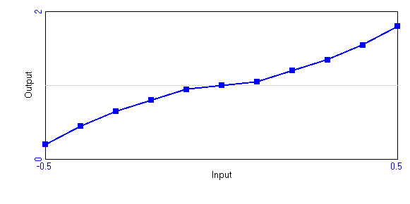
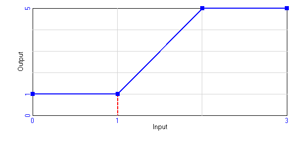
Default	Service Quality	L	Table for Delivered Quality (Dimensionless) = [(-0.5,0)-(0.5,2)],(-0.5,0.2),(-0.4,0.45),(-0.3,0.65),(-0.2,0.8),(-0.1,0.95),(0,1),(0.1,1.05),(0.2,1.2),(0.3,1.35),(0.4,1.55),(0.5,1.8) Description: Non-linear relationship. Delivered quality = f(normalized gap between the actual and expected time per task). Present in 1 view: Service Quailty Used by: Delivered Quality - Service quality is a non-linear relationship between the normalized gap between the actual and expected time per task. The non-linear relationship reflects a flat-response close to 0 to represent the "tolerance zone" of service quality.
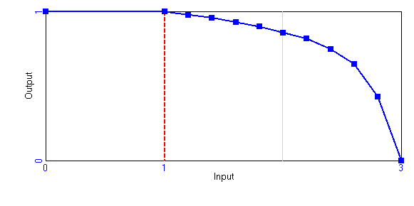
Default	Service Quality	L	Table for Effect of Fatigue on PEF (Dimensionless) = [(0,0)-(3,1)],(0,1),(1,1),(1.2,0.98),(1.4,0.96),(1.6,0.93),(1.8,0.9),(2,0.86),(2.2,0.82),(2.4,0.75),(2.6,0.65),(2.8,0.43),(3,0) Description: Non-linear relationship. Effect of Fatigue on PEF = f(Recent Workweek/Standard Workweek). Present in 1 view: Service Quailty Used by: Effect of Fatigue on Probability of Error Free - The longer the workweek, the more likely it is employees will introduce an error while processing a task.
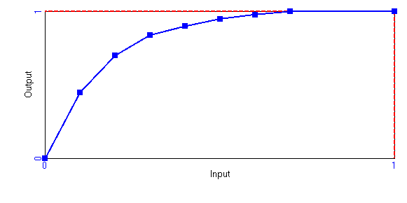
Default	Service Quality	L	Table for Effect of Inexperience on PEF (Dimensionless) = [(0,0)-(1,1)],(0,0),(0.1,0.45),(0.2,0.7),(0.3,0.84),(0.4,0.9),(0.5,0.95),(0.6,0.98),(0.7,1),(1,1) Description: Non-linear relationship. Effect of Inexperience on PEF = f(Average Productivity) Present in 1 view: Service Quailty Used by: Effect of Inexperience on Probability of Error Free - The more experience the workforce has, the less likely they will be of introducing an error while processing a task. Average Productivity is used as a proxy for experience since it captures the amount learning achieved by the workforce.
TOP	Task Flows
Module	*Group*	Type	Variable Name and Description
Default	Task Flows	F,A	Balking Rate (Tasks/Week) = IF THEN ELSE(Market Feedback Switch=1,Service BacklogNormal Balking RateEffect of Delivery Delay on Balking,0) Description: Customers balk at a normal fractional rate modified by the effect of delivery delay. Longer wait times increase the hazard rate of balking. Present in 1 view: Backlog Used by: Service Backlog - The initial backlog is set to the equilibrium value determined by the arrival rate and target delivery delay.
Default	Task Flows	A	Delivery Delay (Weeks) = Service Backlog/Task Completion Rate Description: The average time to complete customer requests is determined by Little's Law as the ratio of the backlog to completion rate. Present in 2 views: Backlog Market Response Used by: Effect of Delivery Delay on Attractiveness - The deviation from the target delivery delay is adjusted by an exponent that reflects how sensitive customers are to these deviations. Effect of Delivery Delay on Balking - There is no balking when delivery delay is normal. When delivery delay rises above some threshold (relative to the normal value), customers begin to balk. The greater the sensitivity of balking to delivery delay, the faster balking increases as wait times grow.
Default	Task Flows	A	Effect of Delivery Delay on Balking (Dimensionless) = MAX(0,((Delivery Delay/(Target Delivery DelayThreshold Delivery Delay for Balking))^Sensitivity of Balking to Delivery Delay)-1) Description:* There is no balking when delivery delay is normal. When delivery delay rises above some threshold (relative to the normal value), customers begin to balk. The greater the sensitivity of balking to delivery delay, the faster balking increases as wait times grow. Present in 2 views: Backlog Market Response Used by: Effect of Balking on Attractiveness - This effect is formulated differently from the other three since the input is already a dimensionless fractional deviation from the desired standard (0). The formulation introduces an acceptable unit error. Balking Rate - Customers balk at a normal fractional rate modified by the effect of delivery delay. Longer wait times increase the hazard rate of balking.
Default	Task Flows	F,A	Error Discovery Rate (Tasks/Week) = Undiscovered Errors/Time to Discover Errors Description: The rate at which errors are discovered by the customer. First order delay from the undiscovered errors stock. Present in 2 views: Backlog Market Response Used by: Effect of Errors on Attractiveness - Targeted error discovery rate is zero. The departure from that goal is relative to the total number of tasks being processed. Service Backlog - The initial backlog is set to the equilibrium value determined by the arrival rate and target delivery delay. Undiscovered Errors - Stock of undiscovered errors.
Default	Task Flows	SI,F,A	Error Generation Rate (Tasks/Week) = IF THEN ELSE(Cutting Corners Switch=1,Task Completion RateProbability of Error Generation,0) Description:* Task with errors generated every week. Present in 1 view: Backlog Used by: Undiscovered Errors - Stock of undiscovered errors.
Default	Task Flows	A	Maximum Completion Rate (Tasks/Week) = Service Backlog/Minimum Delivery Delay Description: The maximum completion rate is determined by the backlog and minimum time to complete a customer request. Present in 1 view: Backlog Used by: Task Completion Rate - The rate at which customer requests are completed is the lesser of the maximum rate or the potential rate, which in turn is determined by labor, workday, and the time spent on each task.
Default	Task Flows	C	Minimum Delivery Delay (Week) = 0.05 Description: The fastest possible completion time for customer requests. Present in 1 view: Backlog Used by: Maximum Completion Rate - The maximum completion rate is determined by the backlog and minimum time to complete a customer request.
Default	Task Flows	C	Normal Balking Rate (1/Week) = 1 Description: The normal balking rate is the hazard rate of balking when delivery delay is Present in 1 view: Backlog Used by: Balking Rate - Customers balk at a normal fractional rate modified by the effect of delivery delay. Longer wait times increase the hazard rate of balking.
Default	Task Flows	C	Sensitivity of Balking to Delivery Delay (Dimensionless [0,20]) = 1.5 Description: Exponent to the Effect of delivery delay on balking. Present in 1 view: Backlog Used by: Effect of Delivery Delay on Balking - There is no balking when delivery delay is normal. When delivery delay rises above some threshold (relative to the normal value), customers begin to balk. The greater the sensitivity of balking to delivery delay, the faster balking increases as wait times grow.
Default	Task Flows	S	Service Backlog (Tasks) = ∫ (Error Discovery Rate+Task Arrival Rate-Balking Rate-Task Completion Rate-Balking Rate) dt + [(Task Arrival Rate)(Target Delivery Delay)] Description:* The initial backlog is set to the equilibrium value determined by the arrival rate and target delivery delay. Present in 1 view: Backlog Used by: Balking Rate - Customers balk at a normal fractional rate modified by the effect of delivery delay. Longer wait times increase the hazard rate of balking. Delivery Delay - The average time to complete customer requests is determined by Little's Law as the ratio of the backlog to completion rate. Maximum Completion Rate - The maximum completion rate is determined by the backlog and minimum time to complete a customer request. Desired Completion Rate - To complete tasks in the target delivery time, the completion rate must be equal to the backlog divided by the target time.
Default	Task Flows	SI,F,A	Task Arrival Rate (Tasks/Week) = IF THEN ELSE(Market Feedback Switch=1,Endogenous Task Arrival Rate, Exogenous Task Arrival Rate) Description: Task Arrivals are set to an exogenous rate. If the market feed back option is active, then the tasks arrival rate depends on the customer base. Present in 1 view: Backlog Used by: Service Backlog - The initial backlog is set to the equilibrium value determined by the arrival rate and target delivery delay.
Default	Task Flows	F,A	Task Completion Rate (Tasks/Week) = MIN(Maximum Completion Rate, Potential Completion Rate) Description: The rate at which customer requests are completed is the lesser of the maximum rate or the potential rate, which in turn is determined by labor, workday, and the time spent on each task. Present in 3 views: Backlog Responses Market Response Used by: Effect of Errors on Attractiveness - Targeted error discovery rate is zero. The departure from that goal is relative to the total number of tasks being processed. Normalized Completion rate - Fractional change of the task completion rate relative to its initial value. It assumes that the model is started in equilibrium and that the initial task completion rate is the same as the arrival rate. Error Generation Rate - Task with errors generated every week. Service Backlog - The initial backlog is set to the equilibrium value determined by the arrival rate and target delivery delay. Delivery Delay - The average time to complete customer requests is determined by Little's Law as the ratio of the backlog to completion rate.
Default	Task Flows	C	Threshold Delivery Delay for Balking (Dimensionless) = 1.002 Description: The greater the threshold (above 1), the higher the delivery delay must be before customers begin to balk as a consequence of long wait times. Present in 1 view: Backlog Used by: Effect of Delivery Delay on Balking - There is no balking when delivery delay is normal. When delivery delay rises above some threshold (relative to the normal value), customers begin to balk. The greater the sensitivity of balking to delivery delay, the faster balking increases as wait times grow.
Default	Task Flows	SI,C	Time to Discover Errors (Week) = 2 Present in 1 view: Backlog Used by: Undiscovered Errors - Stock of undiscovered errors. Error Discovery Rate - The rate at which errors are discovered by the customer. First order delay from the undiscovered errors stock.
Default	Task Flows	S	Undiscovered Errors (Tasks) = ∫ (Error Generation Rate-Error Discovery Rate) dt + [Error Generation RateTime to Discover Errors] Description:* Stock of undiscovered errors. Present in 1 view: Backlog Used by: Error Discovery Rate - The rate at which errors are discovered by the customer. First order delay from the undiscovered errors stock.
TOP	Test Generator for Absenteeism
Module	*Group*	Type	Variable Name and Description
Default	Test Generator for Absenteeism	A	Absenteeism (Dimensionless) = MAX(0, Input 0-1) Description: Absenteeism as a fraction of the labor force is determined by the test generator input for absenteeism (Input 0). Absenteeism is never less than zero (workers often fail to show up for their shift but never show up when they are not scheduled). Present in 1 view: Task Arrivals and Absenteeism
Default	Test Generator for Absenteeism	F,A	Change in Pink Noise 0 (1/Week) = (White Noise 0 - Pink Noise 0)/Noise Correlation Time 0 Description: Change in the pink noise value; Pink noise is a first order exponential smoothing delay of the whitenoise input. Present in 1 view: Task Arrivals and Absenteeism Used by: Pink Noise 0 - Pink Noise is first-order autocorrelated noise. Pink noise provides a realistic noise input tomodels in which the next random shock depends in part on the previous shocks. The usercan specify the correlation time. The mean is 0 and the standard deviation is specifiedby the user.
Default	Test Generator for Absenteeism	A	Input 0 (Dimensionless) = 1+STEP(Step Height 0,Step Time 0)+(Pulse Quantity 0/Pulse Duration 0)PULSE(Pulse Time 0,Pulse Duration 0)+RAMP(Ramp Slope 0,Ramp Start Time 0,Ramp End Time 0)+Sine Amplitude 0SIN(23.14159Time/Sine Period 0)+STEP(1,Noise Start Time 0)Pink Noise 0 Description:* Input is a dimensionless variable which provides a variety of test input patterns, including a step,pulse, sine wave, and random noise. Present in 1 view: Task Arrivals and Absenteeism Used by: Absenteeism - Absenteeism as a fraction of the labor force is determined by the test generator input for absenteeism (Input 0). Absenteeism is never less than zero (workers often fail to show up for their shift but never show up when they are not scheduled).
Default	Test Generator for Absenteeism	C	Noise Correlation Time 0 (Weeks) = 2 Description: The correlation time constant for Pink Noise. Present in 1 view: Task Arrivals and Absenteeism Used by: Change in Pink Noise 0 - Change in the pink noise value; Pink noise is a first order exponential smoothing delay of the whitenoise input. White Noise 0 - White noise input to the pink noise process.
Default	Test Generator for Absenteeism	C	Noise Seed 0 (Dimensionless) = 2 Description: Random number generator seed. Vary to generate a different sequence of random numbers. Present in 1 view: Task Arrivals and Absenteeism
Default	Test Generator for Absenteeism	C	Noise Standard Deviation 0 (Dimensionless) = 0 Description: The standard deviation of the pink noise process. Present in 1 view: Task Arrivals and Absenteeism Used by: White Noise 0 - White noise input to the pink noise process.
Default	Test Generator for Absenteeism	C	Noise Start Time 0 (Week) = 0 Description: Start time for the random input. Present in 1 view: Task Arrivals and Absenteeism Used by: Input 0 - Input is a dimensionless variable which provides a variety of test input patterns, including a step,pulse, sine wave, and random noise.
Default	Test Generator for Absenteeism	S	Pink Noise 0 (Dimensionless) = ∫(Change in Pink Noise 0) dt + [0] Description: Pink Noise is first-order autocorrelated noise. Pink noise provides a realistic noise input tomodels in which the next random shock depends in part on the previous shocks. The usercan specify the correlation time. The mean is 0 and the standard deviation is specifiedby the user. Present in 1 view: Task Arrivals and Absenteeism Used by: Change in Pink Noise 0 - Change in the pink noise value; Pink noise is a first order exponential smoothing delay of the whitenoise input. Input 0 - Input is a dimensionless variable which provides a variety of test input patterns, including a step,pulse, sine wave, and random noise.
Default	Test Generator for Absenteeism	C	Pulse Duration 0 (Week) = 1 Description: Duration of pulse input. Set to Time Step for an impulse. Present in 1 view: Task Arrivals and Absenteeism Used by: Input 0 - Input is a dimensionless variable which provides a variety of test input patterns, including a step,pulse, sine wave, and random noise.
Default	Test Generator for Absenteeism	C	Pulse Quantity 0 (DimensionlessWeek) = 0 Description:* The quantity to be injected to customer orders, as a fraction of the base value of Input.For example, to pulse in a quantity equal to 50% of the current value of input, set to.50. Present in 1 view: Task Arrivals and Absenteeism Used by: Input 0 - Input is a dimensionless variable which provides a variety of test input patterns, including a step,pulse, sine wave, and random noise.
Default	Test Generator for Absenteeism	C	Pulse Time 0 (Week) = 0 Description: Time at which the pulse in Input occurs. Present in 1 view: Task Arrivals and Absenteeism Used by: Input 0 - Input is a dimensionless variable which provides a variety of test input patterns, including a step,pulse, sine wave, and random noise.
Default	Test Generator for Absenteeism	C	Ramp End Time 0 (Week) = 1e+009 Description: End time for the ramp input. Present in 1 view: Task Arrivals and Absenteeism Used by: Input 0 - Input is a dimensionless variable which provides a variety of test input patterns, including a step,pulse, sine wave, and random noise.
Default	Test Generator for Absenteeism	C	Ramp Slope 0 (1/Week) = 0 Description: Slope of the ramp input, as a fraction of the base value (per year). Present in 1 view: Task Arrivals and Absenteeism Used by: Input 0 - Input is a dimensionless variable which provides a variety of test input patterns, including a step,pulse, sine wave, and random noise.
Default	Test Generator for Absenteeism	C	Ramp Start Time 0 (Week) = 0 Description: Start time for the ramp input. Present in 1 view: Task Arrivals and Absenteeism Used by: Input 0 - Input is a dimensionless variable which provides a variety of test input patterns, including a step,pulse, sine wave, and random noise.
Default	Test Generator for Absenteeism	C	Sine Amplitude 0 (Dimensionless) = 0 Description: Amplitude of sine wave in customer orders (fraction of mean). Present in 1 view: Task Arrivals and Absenteeism Used by: Input 0 - Input is a dimensionless variable which provides a variety of test input patterns, including a step,pulse, sine wave, and random noise.
Default	Test Generator for Absenteeism	C	Sine Period 0 (Week) = 52 Description: Period of sine wave in customer demand. Set initially to 52 weeks to simulate annual cycle Present in 1 view: Task Arrivals and Absenteeism Used by: Input 0 - Input is a dimensionless variable which provides a variety of test input patterns, including a step,pulse, sine wave, and random noise.
Default	Test Generator for Absenteeism	C	Step Height 0 (Dimensionless) = 0 Description: Height of step input to customer orders, as fraction of initial value. Present in 1 view: Task Arrivals and Absenteeism Used by: Input 0 - Input is a dimensionless variable which provides a variety of test input patterns, including a step,pulse, sine wave, and random noise.
Default	Test Generator for Absenteeism	C	Step Time 0 (Weeks) = 0 Description: Time for the step input. Present in 1 view: Task Arrivals and Absenteeism Used by: Input 0 - Input is a dimensionless variable which provides a variety of test input patterns, including a step,pulse, sine wave, and random noise.
Default	Test Generator for Absenteeism	A	White Noise 0 (Dimensionless) = Noise Standard Deviation 0((24Noise Correlation Time 0/TIME STEP)^0.5(RANDOM 0 1 - 0.5)) Description:* White noise input to the pink noise process. Present in 1 view: Task Arrivals and Absenteeism Used by: Change in Pink Noise 0 - Change in the pink noise value; Pink noise is a first order exponential smoothing delay of the whitenoise input.
TOP	Test Generator for Arrivals
Module	*Group*	Type	Variable Name and Description
Default	Test Generator for Arrivals	F,A	Change in Pink Noise (1/Week) = (White Noise - Pink Noise)/Noise Correlation Time Description: Change in the pink noise value; Pink noise is a first order exponential smoothing delay of the whitenoise input. Present in 1 view: Task Arrivals and Absenteeism Used by: Pink Noise - Pink Noise is first-order autocorrelated noise. Pink noise provides a realistic noise input tomodels in which the next random shock depends in part on the previous shocks. The usercan specify the correlation time. The mean is 0 and the standard deviation is specifiedby the user.
Default	Test Generator for Arrivals	I	Exogenous Task Arrival Rate (Tasks/Week) = Initial Arrival RateInput Description:* The exogenous task arrival rate can be configured to include a range of test inputs. It is set to the product of the initial arrival rate and the test input. The test input allows users to specify a range of input patterns, including a step, pulse, ramp, cycle, and pink noise, or combinations of these. Present in 2 views: Backlog Task Arrivals and Absenteeism Used by: Task Arrival Rate - Task Arrivals are set to an exogenous rate. If the market feed back option is active, then the tasks arrival rate depends on the customer base.
Default	Test Generator for Arrivals	I	Initial Arrival Rate (Tasks/Week) = INITIAL(Standard Completion Rate) Description: The initial rate at which work arrives is set to the initial value of the standard completion rate. Note that the equation type is INITIAL, which ensures that the initial arrival rate remains constant even if the standard completion rate varies. By setting the initial arrival rate to the standard completion rate we ensure that tasks arrive at exactly the rate the organization can handle given the initial staff and standard values for the workday and time per task. Present in 2 views: Task Arrivals and Absenteeism Responses Used by: Normalized Completion rate - Fractional change of the task completion rate relative to its initial value. It assumes that the model is started in equilibrium and that the initial task completion rate is the same as the arrival rate. Exogenous Task Arrival Rate - The exogenous task arrival rate can be configured to include a range of test inputs. It is set to the product of the initial arrival rate and the test input. The test input allows users to specify a range of input patterns, including a step, pulse, ramp, cycle, and pink noise, or combinations of these.
Default	Test Generator for Arrivals	A	Input (Dimensionless) = 1+STEP(Step Height,Step Time)+(Pulse Quantity/Pulse Duration)PULSE(Pulse Time,Pulse Duration)+RAMP(Ramp Slope,Ramp Start Time,Ramp End Time)+Sine AmplitudeSIN(23.14159Time/Sine Period)+STEP(1,Noise Start Time)Pink Noise Description:* Input is a dimensionless variable which provides a variety of test input patterns, including a step,pulse, sine wave, and random noise. Present in 2 views: Task Arrivals and Absenteeism Market Response Used by: Endogenous Task Arrival Rate - Note that the impact of the input on the endogenous task arrival rate would be equivalent to modifying the task request per customer since the base line would be affected by changes in the customer base. Exogenous Task Arrival Rate - The exogenous task arrival rate can be configured to include a range of test inputs. It is set to the product of the initial arrival rate and the test input. The test input allows users to specify a range of input patterns, including a step, pulse, ramp, cycle, and pink noise, or combinations of these.
Default	Test Generator for Arrivals	C	Noise Correlation Time (Week) = 4 Description: The correlation time constant for Pink Noise. Present in 1 view: Task Arrivals and Absenteeism Used by: Change in Pink Noise - Change in the pink noise value; Pink noise is a first order exponential smoothing delay of the whitenoise input. White Noise - White noise input to the pink noise process.
Default	Test Generator for Arrivals	C	Noise Seed (Dimensionless) = 70 Description: Random number generator seed. Vary to generate a different sequence of random numbers. Present in 1 view: Task Arrivals and Absenteeism
Default	Test Generator for Arrivals	C	Noise Standard Deviation (Dimensionless) = 0.1 Description: The standard deviation of the pink noise process. Present in 1 view: Task Arrivals and Absenteeism Used by: White Noise - White noise input to the pink noise process.
Default	Test Generator for Arrivals	C	Noise Start Time (Week) = 10 Description: Start time for the random input. Present in 1 view: Task Arrivals and Absenteeism Used by: Input - Input is a dimensionless variable which provides a variety of test input patterns, including a step,pulse, sine wave, and random noise.
Default	Test Generator for Arrivals	S	Pink Noise (Dimensionless) = ∫(Change in Pink Noise) dt + [0] Description: Pink Noise is first-order autocorrelated noise. Pink noise provides a realistic noise input tomodels in which the next random shock depends in part on the previous shocks. The usercan specify the correlation time. The mean is 0 and the standard deviation is specifiedby the user. Present in 1 view: Task Arrivals and Absenteeism Used by: Change in Pink Noise - Change in the pink noise value; Pink noise is a first order exponential smoothing delay of the whitenoise input. Input - Input is a dimensionless variable which provides a variety of test input patterns, including a step,pulse, sine wave, and random noise.
Default	Test Generator for Arrivals	C	Pulse Duration (Week) = 13 Description: Duration of pulse input. Set to Time Step for an impulse. Present in 1 view: Task Arrivals and Absenteeism Used by: Input - Input is a dimensionless variable which provides a variety of test input patterns, including a step,pulse, sine wave, and random noise.
Default	Test Generator for Arrivals	C	Pulse Quantity (DimensionlessWeek) = 0 Description:* The quantity to be injected to customer orders, as a fraction of the base value of Input.For example, to pulse in a quantity equal to 50% of the current value of input, set to.50. Present in 1 view: Task Arrivals and Absenteeism Used by: Input - Input is a dimensionless variable which provides a variety of test input patterns, including a step,pulse, sine wave, and random noise.
Default	Test Generator for Arrivals	C	Pulse Time (Week) = 10 Description: Time at which the pulse in Input occurs. Present in 1 view: Task Arrivals and Absenteeism Used by: Input - Input is a dimensionless variable which provides a variety of test input patterns, including a step,pulse, sine wave, and random noise.
Default	Test Generator for Arrivals	C	Ramp End Time (Week) = 1e+009 Description: End time for the ramp input. Present in 1 view: Task Arrivals and Absenteeism Used by: Input - Input is a dimensionless variable which provides a variety of test input patterns, including a step,pulse, sine wave, and random noise.
Default	Test Generator for Arrivals	C	Ramp Slope (1/Week) = 0 Description: Slope of the ramp input, as a fraction of the base value (per week). Present in 1 view: Task Arrivals and Absenteeism Used by: Input - Input is a dimensionless variable which provides a variety of test input patterns, including a step,pulse, sine wave, and random noise.
Default	Test Generator for Arrivals	C	Ramp Start Time (Week) = 0 Description: Start time for the ramp input. Present in 1 view: Task Arrivals and Absenteeism Used by: Input - Input is a dimensionless variable which provides a variety of test input patterns, including a step,pulse, sine wave, and random noise.
Default	Test Generator for Arrivals	C	Sine Amplitude (Dimensionless) = 0 Description: Amplitude of sine wave in customer orders (fraction of mean). Present in 1 view: Task Arrivals and Absenteeism Used by: Input - Input is a dimensionless variable which provides a variety of test input patterns, including a step,pulse, sine wave, and random noise.
Default	Test Generator for Arrivals	C	Sine Period (Week) = 52 Description: Period of sine wave in customer demand. Set initially to 52 weeks to simulate an annual cycle Present in 1 view: Task Arrivals and Absenteeism Used by: Input - Input is a dimensionless variable which provides a variety of test input patterns, including a step,pulse, sine wave, and random noise.
Default	Test Generator for Arrivals	C	Step Height (Dimensionless) = 0 Description: Height of step input to customer orders, as fraction of initial value. Present in 1 view: Task Arrivals and Absenteeism Used by: Input - Input is a dimensionless variable which provides a variety of test input patterns, including a step,pulse, sine wave, and random noise.
Default	Test Generator for Arrivals	C	Step Time (Week) = 10 Description: Time for the step input. Present in 1 view: Task Arrivals and Absenteeism Used by: Input - Input is a dimensionless variable which provides a variety of test input patterns, including a step,pulse, sine wave, and random noise.
Default	Test Generator for Arrivals	A	White Noise (Dimensionless) = Noise Standard Deviation((24Noise Correlation Time/TIME STEP)^0.5(RANDOM 0 1 - 0.5)) Description:* White noise input to the pink noise process. Present in 1 view: Task Arrivals and Absenteeism Used by: Change in Pink Noise - Change in the pink noise value; Pink noise is a first order exponential smoothing delay of the whitenoise input.
TOP	Test Switches
Module	*Group*	Type	Variable Name and Description
Default	Test Switches	C	Capacity Switch (Dimensionless) = 1 Description: Switch to control whether the capacity response is active. Present in 1 view: Workforce Used by: Rookie Hire Rate - Replaces the total quit rate and increases total personnel according to the specified growth rate and test option.
Default	Test Switches	C	Cutting Corners Switch (Dimensionless) = 1 Description: Switch to control if the cutting corners response is active. Present in 1 view: Backlog Used by: Error Generation Rate - Task with errors generated every week. Effect of Work Pressure on Time per Task - High schedule pressure reduces the time spent on each task.
Default	Test Switches	C	Financial Switch (Dimensionless [0,1,1]) = 1 Description: Switch to control if financial feedback is active. Present in 1 view: Effective, Desired and Authorized Workforce Used by: Authorized Workforce - Authorized workforce is the Minimum of the Desired Workforce to process orders and the Affordable Workforce based on budget constraints
Default	Test Switches	C	Market Feedback Switch (Dimensionless) = 1 Description: Switch to control if market feedback loops are active, i.e., if the task arrival rate is endogenously generated or not. Present in 1 view: Backlog Used by: Balking Rate - Customers balk at a normal fractional rate modified by the effect of delivery delay. Longer wait times increase the hazard rate of balking. Task Arrival Rate - Task Arrivals are set to an exogenous rate. If the market feed back option is active, then the tasks arrival rate depends on the customer base.
Default	Test Switches	C	Step test switch (Dimensionless) = 0 Description: Switch to control whether the growth rate will be treated as Compound Annual Growth Rate, or as a fraction step increase on total personnel. Note that this is switch that introduces a step input, unlike the other switches that activate/de-activate elements of the model structure. Present in 1 view: Workforce Used by: Rookie Hire Rate - Replaces the total quit rate and increases total personnel according to the specified growth rate and test option.
Default	Test Switches	C	Workweek Switch (Dimensionless) = 1 Description: Switch to control if the workweek response is active. Present in 1 view: Backlog Used by: Effect of Work Pressure on Workweek - High schedule pressure leads to overtime; low pressure to a reduction in hours worked.
TOP	Time per Task
Module	*Group*	Type	Variable Name and Description
Default	Time per Task	A	Adjustment Time for Standard Time Per Task (Week) = IF THEN ELSE(Time per Task>Standard Time per Task, Time to Increase Standard Time per Task, Time to Decrease Standard Time per Task) Description: The norm for standard time per task adjusts to the actual time spent on tasks. The speed of adjustment differs when time per task is less than the standard vs more than the standard. Management interprets lower times as productivity improvements and rewards them; increases are viewed as costly deviations. Present in 1 view: Standard Time per Task Used by: Change in Standard Time per Task - The standard time per task adjusts gradually toward the actual time workers spend on tasks.
Default	Time per Task	F,A	Change in Standard Time per Task (PersonHours/(WeekTask)) = (Time per Task - Standard Time per Task)/Adjustment Time for Standard Time Per Task Description: The standard time per task adjusts gradually toward the actual time workers spend on tasks. Present in 2 views: Backlog Standard Time per Task Used by: Standard Time per Task - The standard time spent on each task (in person-hours/task) is the time workers believe should be allocated to each task when schedule pressure is normal.
Default	Time per Task	A	Effect of Work Pressure on Time per Task (Dimensionless) = IF THEN ELSE( Cutting Corners Switch=1,Table for Effect of Work Pressure on Time per Task(Work Pressure),1) Description: High schedule pressure reduces the time spent on each task. Present in 1 view: Backlog Used by: Time per Task - The actual time spent on each task is the standard time modified by the effect of schedule pressure. High pressure reduces the time per task.
Default	Time per Task	SI,C	Initial Standard Time per Task (Personhour/Task) = 1 Description:* Initial value of the Standard Time per Task. Present in 4 views: Backlog Standard Time per Task Service Quailty Responses Used by: Normalized Standard Time per Task - Fractional change of the Standard Time per Task relative to its initial value. Customer Expected Time Per Task - Reference point for customer expectations. Set to Initial Standard Time per Task to start the model in equilibrium. Standard Time per Task - The standard time spent on each task (in person-hours/task) is the time workers believe should be allocated to each task when schedule pressure is normal.
Default	Time per Task	S	Standard Time per Task (PersonHours/Task) = ∫ (Change in Standard Time per Task) dt + [Initial Standard Time per Task] Description:* The standard time spent on each task (in person-hours/task) is the time workers believe should be allocated to each task when schedule pressure is normal. Present in 3 views: Backlog Standard Time per Task Responses Used by: Standard Completion Rate - The standard completion rate is the rate at which tasks would be completed by the current workforce at the standard workday and spending the standard time on each task. Used to initialize the market sector in equilibrium. Normalized Time per Task - Fractional change of the Time per Task relative to the Standard Time per Task. Note that the Standard Time per Task is a variable, as opposed to the other references for the responses to work pressure that are all constant. Thus, the total adjustment of Time per Task is it change relative to the Standard, and the change of the Standard relative to its initial value. Normalized Standard Time per Task - Fractional change of the Standard Time per Task relative to its initial value. Change in Standard Time per Task - The standard time per task adjusts gradually toward the actual time workers spend on tasks. Adjustment Time for Standard Time Per Task - The norm for standard time per task adjusts to the actual time spent on tasks. The speed of adjustment differs when time per task is less than the standard vs more than the standard. Management interprets lower times as productivity improvements and rewards them; increases are viewed as costly deviations. Time per Task - The actual time spent on each task is the standard time modified by the effect of schedule pressure. High pressure reduces the time per task. Desired Service Capacity - This is the required service capacity based on the desired production rate and the standard work intensity and time allocation.
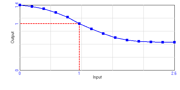
Default	Time per Task	L	Table for Effect of Work Pressure on Time per Task (Dimensionless) = [(0,0)-(2.6,1.4)],(0,1.4),(0.2,1.37),(0.4,1.32),(0.6,1.24),(0.8,1.14),(1,1),(1.2,0.89),(1.4,0.79),(1.6,0.7),(1.8,0.65),(2,0.62),(2.2,0.61),(2.4,0.6),(2.6,0.6) Description: High schedule pressure leads to corner cutting and less time per task. Present in 1 view: Backlog Used by: Effect of Work Pressure on Time per Task - High schedule pressure reduces the time spent on each task.
Default	Time per Task	A	Time per Task (Personhour/Task) = Standard Time per TaskEffect of Work Pressure on Time per Task Description: The actual time spent on each task is the standard time modified by the effect of schedule pressure. High pressure reduces the time per task. Present in 4 views: Backlog Standard Time per Task Service Quailty Responses Used by: Normalized Time per Task - Fractional change of the Time per Task relative to the Standard Time per Task. Note that the Standard Time per Task is a variable, as opposed to the other references for the responses to work pressure that are all constant. Thus, the total adjustment of Time per Task is it change relative to the Standard, and the change of the Standard relative to its initial value. Effect of Time per Order on Probability of Error Free - The less time employees allocate to each task, the more likely they will be of introducing an error while processing the task. The formulation introduces a MIN to represent the effect that allocating more time per task will not increase the probability of an error free task beyond one. Delivered Quality - Service quality is a non-linear relationship between the normalized gap between the actual and expected time per task. The non-linear relationship reflects a flat-response close to 0 to represent the "tolerance zone" of service quality. Change in Standard Time per Task - The standard time per task adjusts gradually toward the actual time workers spend on tasks. Adjustment Time for Standard Time Per Task - The norm for standard time per task adjusts to the actual time spent on tasks. The speed of adjustment differs when time per task is less than the standard vs more than the standard. Management interprets lower times as productivity improvements and rewards them; increases are viewed as costly deviations. Potential Completion Rate - The potential completion rate depends on the net available labor force, the workday, and the average time spent on each task.
Default	Time per Task	C	Time to Decrease Standard Time per Task (Week) = 20 Description: The time period over which standard time per task adjusts to actual time per task. Present in 1 view: Standard Time per Task Used by: Adjustment Time for Standard Time Per Task - The norm for standard time per task adjusts to the actual time spent on tasks. The speed of adjustment differs when time per task is less than the standard vs more than the standard. Management interprets lower times as productivity improvements and rewards them; increases are viewed as costly deviations.
Default	Time per Task	C	Time to Increase Standard Time per Task (Week) = 30 Description: The time period over which the norm for standard time per task increases. Present in 1 view: Standard Time per Task Used by: Adjustment Time for Standard Time Per Task - The norm for standard time per task adjusts to the actual time spent on tasks. The speed of adjustment differs when time per task is less than the standard vs more than the standard. Management interprets lower times as productivity improvements and rewards them; increases are viewed as costly deviations.
Default	Time per Task	A	Work Pressure (Dimensionless) = Desired Service Capacity/Service Capacity Description: Work pressure is the ratio of the desired to standard service capacity. Present in 1 view: Backlog Used by: Effect of Work Pressure on Time per Task - High schedule pressure reduces the time spent on each task. Effect of Work Pressure on Workweek - High schedule pressure leads to overtime; low pressure to a reduction in hours worked.
TOP	Workforce
Module	*Group*	Type	Variable Name and Description
Default	Workforce	F,A	Assimilation Rate (Employees/Week) = Rookie Employees/Assimilation Time Description: Rate of employees gaining full productivity. Present in 1 view: Workforce Used by: Experienced Employees - Employees that have achieved full productivity. Rookie Employees - Recently hired employees that have not achieved full productivity.
Default	Workforce	C	Assimilation Time (Week [0,250]) = 50 Description: Average time required to achieve the productivity of a Fully Trained employee. Present in 2 views: Workforce Effective, Desired and Authorized Workforce Used by: LC AR - Assimilation rate for the individual learning curve. Assimilation Rate - Rate of employees gaining full productivity. Steady State Rookie Fraction - Rookie fraction in equilibrium, or steady state growth. Used to initialize the model.
Default	Workforce	A	Average Productivity (Dimensionless) = Effective Workforce/Total Employees Description: Average productivity for Total personnel. Present in 2 views: Effective, Desired and Authorized Workforce Service Quailty Used by: Effect of Inexperience on Probability of Error Free - The more experience the workforce has, the less likely they will be of introducing an error while processing a task. Average Productivity is used as a proxy for experience since it captures the amount learning achieved by the workforce.
Default	Workforce	A	Desired Hiring Rate (Employees/Week) = Replacement Rate+Workforce Adjustment Rate Description: The desired hiring rate replaces employees that left the firm and adjust for changes in the desired workforce. Present in 1 view: Workforce Used by: Desired Vacancies - Desired number of vacancies to maintain the desired hiring rate (from Little's law). Indicated Labor Order Rate - Indicated number of vacancies to be created or cancelled.
Default	Workforce	SI,A	Desired Vacancies (Employees) = Desired Hiring RateTime to Hire Description:* Desired number of vacancies to maintain the desired hiring rate (from Little's law). Present in 1 view: Workforce Used by: Employee Vacancies - The total number of authorized positions that have not been filled yet. Vacancy Adjustment Rate - Vacancies that have to be created or destroyed to reach the desired vacancies over the time to adjust the workforce.
Default	Workforce	A	Effect of Burnout on Turnover (Dimensionless) = Table for Effect of Burnout on Turnover(Long Term Workweek/Standard Workweek) Description: The higher the workweek, the higher the turnover rate. The accumulation of the workweek happens over a period of 52 weeks. Present in 1 view: Workforce Used by: Experienced Quit Rate - Experienced employees turnover. Rookie Quit Rate - Rookie turnover rate.
Default	Workforce	A	Effect of Quality on Turnover (Dimensionless) = Table for Effect of Quality on Turnover(Delivered Quality) Description: The higher the service quality, the lower the turnover rate. Employees will be more loyal to the firm if they perceive the are delivering good quality to the customer. Present in 1 view: Workforce Used by: Experienced Quit Rate - Experienced employees turnover. Rookie Quit Rate - Rookie turnover rate.
Default	Workforce	A	Effective Experienced employees (Employees) = MAX(0,Experienced Employees-Rookie EmployeesFraction of time required to train rookies) Description:* Experienced employees available to perform productive work after training rookies. Effective experienced employees is limited to 0 to avoid the utilization of resources not available for training. The model, however, does not consider secondary effects, i.e., extending the assimilation time, due to the lack of mentors. Present in 1 view: Effective, Desired and Authorized Workforce Used by: Effective Workforce - Expected output from the labor pool accounting for labor mix and the impact of mentoring on Experienced employees' productivity. Measured in FTE (Fully Trained Equivalents). Experienced fraction to training - Fraction of Experienced employees' time that is being allocated to train rookies. IF THEN ELSE condition introduced to eliminate potential division-by-zero error in case the model is initialized with all-rookie labor force.
Default	Workforce	A	Effective Workforce (Employees) = (Effective Experienced employees+Rookie EmployeesRookie productivity fraction) Description:* Expected output from the labor pool accounting for labor mix and the impact of mentoring on Experienced employees' productivity. Measured in FTE (Fully Trained Equivalents). Present in 3 views: Effective, Desired and Authorized Workforce Backlog Responses Used by: Initial Effective Workforce - Initial value of the Effective workforce. Used to calculate the fractional change in the workforce effectiveness. Normalized Effective Workforce - Fractional change of the Effective workforce relative to its initial value. Service Capacity - The workforce effectiveness is affected by the accumulated fatigue resulting from extended workweeks. Average Productivity - Average productivity for Total personnel.
Default	Workforce	S	Employee Vacancies (Employees) = ∫ (Labor Order Rate-Hiring Rate) dt + [Desired Vacancies] Description: The total number of authorized positions that have not been filled yet. Present in 1 view: Workforce Used by: Hiring Rate - Hiring rate is the first order delay of the vacancies that have been created. Labor Order Rate - Number of vacancies created or cancelled. The MAX condition ensures that only existing vacancies can be cancelled. Vacancy Adjustment Rate - Vacancies that have to be created or destroyed to reach the desired vacancies over the time to adjust the workforce.
Default	Workforce	S	Experienced Employees (Employees) = ∫ (Assimilation Rate-Experienced Quit Rate) dt + [Initial employees(1-Steady State Rookie Fraction)] Description:* Employees that have achieved full productivity. Present in 2 views: Workforce Effective, Desired and Authorized Workforce Used by: Experienced Quit Rate - Experienced employees turnover. Effective Experienced employees - Experienced employees available to perform productive work after training rookies. Effective experienced employees is limited to 0 to avoid the utilization of resources not available for training. The model, however, does not consider secondary effects, i.e., extending the assimilation time, due to the lack of mentors. Experienced fraction to training - Fraction of Experienced employees' time that is being allocated to train rookies. IF THEN ELSE condition introduced to eliminate potential division-by-zero error in case the model is initialized with all-rookie labor force. Total Employees - Total employees.
Default	Workforce	A	Experienced fraction to training (Dimensionless) = IF THEN ELSE(Experienced Employees=0,1 , (Experienced Employees-Effective Experienced employees)/Experienced Employees) Description: Fraction of Experienced employees' time that is being allocated to train rookies. IF THEN ELSE condition introduced to eliminate potential division-by-zero error in case the model is initialized with all-rookie labor force. Present in 1 view: Effective, Desired and Authorized Workforce Used by: This is a supplementary variable.
Default	Workforce	C	Experienced Quit Fraction (Dimensionless/Week [0,2]) = 0.004 Description: Fraction of Experienced employees that leaves the firm every week. Present in 1 view: Workforce Used by: Experienced Quit Rate - Experienced employees turnover. Steady State Rookie Fraction - Rookie fraction in equilibrium, or steady state growth. Used to initialize the model.
Default	Workforce	F,A	Experienced Quit Rate (Employees/Week) = Experienced EmployeesExperienced Quit FractionEffect of Burnout on TurnoverEffect of Quality on Turnover Description:* Experienced employees turnover. Present in 1 view: Workforce Used by: Experienced Employees - Employees that have achieved full productivity. Total Quit Rate - Total turnover rate.
Default	Workforce	C	Fraction of time required to train rookies (Dimensionless [0,1]) = 0.1 Description: Fraction of an Experienced employee's time required to train/mentor one rookie. This fraction of time is allocated throughout the period before a rookie is fully assimilated. Present in 1 view: Effective, Desired and Authorized Workforce Used by: Effective Experienced employees - Experienced employees available to perform productive work after training rookies. Effective experienced employees is limited to 0 to avoid the utilization of resources not available for training. The model, however, does not consider secondary effects, i.e., extending the assimilation time, due to the lack of mentors.
Default	Workforce	C	Growth Rate (Dimensionless/Week [-1,2]) = 0 Description: Depending on the position of the step test switch, it works as a fractional Step Input or as Compound Annual Growth Rate. Present in 1 view: Workforce Used by: Rookie Hire Rate - Replaces the total quit rate and increases total personnel according to the specified growth rate and test option. Steady State Rookie Fraction - Rookie fraction in equilibrium, or steady state growth. Used to initialize the model.
Default	Workforce	F,A	Hiring Rate (Employees/Week) = Employee Vacancies/Time to Hire Description: Hiring rate is the first order delay of the vacancies that have been created. Present in 1 view: Workforce Used by: Employee Vacancies - The total number of authorized positions that have not been filled yet. Rookie Hire Rate - Replaces the total quit rate and increases total personnel according to the specified growth rate and test option.
Default	Workforce	A	Indicated Labor Order Rate (Employees/Week) = Desired Hiring Rate+Vacancy Adjustment Rate Description: Indicated number of vacancies to be created or cancelled. Present in 1 view: Workforce Used by: Labor Order Rate - Number of vacancies created or cancelled. The MAX condition ensures that only existing vacancies can be cancelled.
Default	Workforce	SI,C	Initial employees (Employees) = 200 Description: Initial number of employees. This parameter sizes the workforce. Individual stocks will be initiated in equilibrium. Present in 1 view: Workforce Used by: Experienced Employees - Employees that have achieved full productivity. Rookie Employees - Recently hired employees that have not achieved full productivity.
Default	Workforce	F,A	Labor Order Rate (Employees/Week) = MAX(-Employee Vacancies/Time to Cancel Vacancies,Indicated Labor Order Rate) Description: Number of vacancies created or cancelled. The MAX condition ensures that only existing vacancies can be cancelled. Present in 1 view: Workforce Used by: Employee Vacancies - The total number of authorized positions that have not been filled yet.
Default	Workforce	A	Replacement Rate (Employees/Week) = Total Quit Rate Description: Employee replacement rate is equal to the total employee turnover rate. Present in 1 view: Workforce Used by: Desired Hiring Rate - The desired hiring rate replaces employees that left the firm and adjust for changes in the desired workforce.
Default	Workforce	S	Rookie Employees (Employees) = ∫ (+Rookie Hire Rate-Assimilation Rate-Rookie Quit Rate) dt + [Initial employeesSteady State Rookie Fraction] Description:* Recently hired employees that have not achieved full productivity. Present in 2 views: Workforce Effective, Desired and Authorized Workforce Used by: Rookie Quit Rate - Rookie turnover rate. Assimilation Rate - Rate of employees gaining full productivity. Effective Workforce - Expected output from the labor pool accounting for labor mix and the impact of mentoring on Experienced employees' productivity. Measured in FTE (Fully Trained Equivalents). Effective Experienced employees - Experienced employees available to perform productive work after training rookies. Effective experienced employees is limited to 0 to avoid the utilization of resources not available for training. The model, however, does not consider secondary effects, i.e., extending the assimilation time, due to the lack of mentors. Rookie fraction - Fraction of employees that have not been fully trained. Total Employees - Total employees.
Default	Workforce	A	Rookie fraction (Dimensionless) = Rookie Employees/Total Employees Description: Fraction of employees that have not been fully trained. Present in 1 view: Workforce Used by: This is a supplementary variable.
Default	Workforce	F,A	Rookie Hire Rate (Employees/Week) = IF THEN ELSE(Capacity Switch=1, Hiring Rate , Total Quit Rate+IF THEN ELSE( Step test switch=1 ,Total EmployeesGrowth RatePULSE(0.5, 0.125 )/0.125 , Total EmployeesGrowth Rate)) Description:* Replaces the total quit rate and increases total personnel according to the specified growth rate and test option. Present in 1 view: Workforce Used by: Rookie Employees - Recently hired employees that have not achieved full productivity.
Default	Workforce	C	Rookie productivity fraction (Dimensionless [-1,1]) = 0.3 Description: Initial rookie productivity ÐÐ measured as a fraction of the productivity of a Fully Trained Employee. Present in 1 view: Effective, Desired and Authorized Workforce Used by: LC - Average individual learning curve. Created exclusively for reporting purposes. Estimates the individual learning curve by reporting the productivity of a single individual as it makes the transition from rookie to experienced employee. Formulation is equivalent to workforce productivity, but limited to a single employee and with no effects from hiring and turnover rates, Effective Workforce - Expected output from the labor pool accounting for labor mix and the impact of mentoring on Experienced employees' productivity. Measured in FTE (Fully Trained Equivalents).
Default	Workforce	C	Rookie Quit Fraction (Dimensionless/Week [0,2]) = 0 Description: Fraction of rookie employees that leaves the firm every week. Present in 1 view: Workforce Used by: Rookie Quit Rate - Rookie turnover rate.
Default	Workforce	F,A	Rookie Quit Rate (Employees/Week) = Rookie EmployeesRookie Quit FractionEffect of Burnout on TurnoverEffect of Quality on Turnover Description:* Rookie turnover rate. Present in 1 view: Workforce Used by: Rookie Employees - Recently hired employees that have not achieved full productivity. Total Quit Rate - Total turnover rate.
Default	Workforce	SI,A	Steady State Rookie Fraction (Dimensionless) = Assimilation Time(Experienced Quit Fraction+Growth Rate)/(1+Assimilation Time(Experienced Quit Fraction+Growth Rate)) Description: Rookie fraction in equilibrium, or steady state growth. Used to initialize the model. Present in 1 view: Workforce Used by: Experienced Employees - Employees that have achieved full productivity. Rookie Employees - Recently hired employees that have not achieved full productivity.
Default	Workforce	L	Table for Effect of Burnout on Turnover (Dimensionless) = [(0,0)-(3,5)],(0,1),(1,1),(2,5),(3,5) Description: The higher the burnout (higher average work week over a period of 52 weeks) the higher the turnover rate. Present in 1 view: Workforce Used by: Effect of Burnout on Turnover - The higher the workweek, the higher the turnover rate. The accumulation of the workweek happens over a period of 52 weeks.
Default	Workforce	L	Table for Effect of Quality on Turnover (Dimensionless) = [(0,0)-(3,3)],(0,3),(0.2,2.85),(0.4,2.5),(0.6,2),(0.7,1.7),(0.9,1.2),(1,1),(1.1,0.8),(1.3,0.6),(1.6,0.53),(2,0.5),(3,0.5) Description: Non-linear effect of delivered quality on the employee turnover rate. Present in 1 view: Workforce Used by: Effect of Quality on Turnover - The higher the service quality, the lower the turnover rate. Employees will be more loyal to the firm if they perceive the are delivering good quality to the customer.
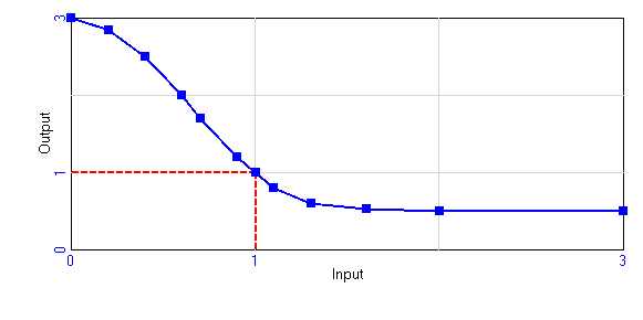
Default	Workforce	C	Time to Adjust Workforce (Week) = 11 Description: Time to adjust the workforce. Set to 11 weeks based on NatWest data. Present in 1 view: Workforce Used by: Workforce Adjustment Rate - Adjustments to the workforce. Smoothed over the time to adjust workforce. Vacancy Adjustment Rate - Vacancies that have to be created or destroyed to reach the desired vacancies over the time to adjust the workforce.
Default	Workforce	C	Time to Cancel Vacancies (Week) = 1 Description: Time to Adjust workforce Present in 1 view: Workforce Used by: Labor Order Rate - Number of vacancies created or cancelled. The MAX condition ensures that only existing vacancies can be cancelled.
Default	Workforce	C	Time to Hire (Week) = 30 Description: Time it takes to advertise the position, and interview, select and recruit a candidate. Set to 30 weeks based on NatWest data. Present in 1 view: Workforce Used by: Desired Vacancies - Desired number of vacancies to maintain the desired hiring rate (from Little's law). Hiring Rate - Hiring rate is the first order delay of the vacancies that have been created.
Default	Workforce	A	Total Employees (Employees) = Rookie Employees+Experienced Employees Description: Total employees. Present in 2 views: Workforce Effective, Desired and Authorized Workforce Used by: Workforce Adjustment Rate - Adjustments to the workforce. Smoothed over the time to adjust workforce. Rookie Hire Rate - Replaces the total quit rate and increases total personnel according to the specified growth rate and test option. Average Productivity - Average productivity for Total personnel. Rookie fraction - Fraction of employees that have not been fully trained. Base Budget - Initialization value for the Base Budget, determined as the fraction of the payroll not covered by operational revenue. Perceived Employee Effectiveness - Management perception of workforce effectiveness. Note that this is an aggregate measure that does not distinguish the employees experience, nor the effects of fatigue, work intensity, or time per task.
Default	Workforce	A	Total Quit Rate (Employees/Week) = Rookie Quit Rate+Experienced Quit Rate Description: Total turnover rate. Present in 1 view: Workforce Used by: Replacement Rate - Employee replacement rate is equal to the total employee turnover rate. Rookie Hire Rate - Replaces the total quit rate and increases total personnel according to the specified growth rate and test option.
Default	Workforce	A	Vacancy Adjustment Rate (Employees/Week) = (Desired Vacancies-Employee Vacancies)/Time to Adjust Workforce Description: Vacancies that have to be created or destroyed to reach the desired vacancies over the time to adjust the workforce. Present in 1 view: Workforce Used by: Indicated Labor Order Rate - Indicated number of vacancies to be created or cancelled.
Default	Workforce	A	Workforce Adjustment Rate (Employees/Week) = (Authorized Workforce-Total Employees)/Time to Adjust Workforce Description: Adjustments to the workforce. Smoothed over the time to adjust workforce. Present in 1 view: Workforce Used by: Desired Hiring Rate - The desired hiring rate replaces employees that left the firm and adjust for changes in the desired workforce.
TOP	Workforce Planning
Module	*Group*	Type	Variable Name and Description
Default	Workforce Planning	SM	Affordable Workforce (Employees) = SMOOTH(Budget/Cost per Employee, Time to Adjust Affordable Workforce ) Description: Number of employees that would be possible to hire as per the budget constraint. Present in 1 view: Effective, Desired and Authorized Workforce Used by: Authorized Workforce - Authorized workforce is the Minimum of the Desired Workforce to process orders and the Affordable Workforce based on budget constraints
Default	Workforce Planning	A	Authorized Workforce (Employees) = (IF THEN ELSE(Financial Switch=1, MIN(Desired Workforce,Affordable Workforce) , Desired Workforce)) Description: Authorized workforce is the Minimum of the Desired Workforce to process orders and the Affordable Workforce based on budget constraints Present in 2 views: Workforce Effective, Desired and Authorized Workforce Used by: Workforce Adjustment Rate - Adjustments to the workforce. Smoothed over the time to adjust workforce.
Default	Workforce Planning	I	Base Budget ($/Week) = INITIAL(Total EmployeesCost per Employee-Fraction of Revenue for OperationsRevenue) Description: Initialization value for the Base Budget, determined as the fraction of the payroll not covered by operational revenue. Present in 1 view: Effective, Desired and Authorized Workforce Used by: Budget - Budget for the workforce. It has a fixed components (base budget) and a variable component depending on the revenue generated. This budget is adjusted by the Margin for Reserve Capacity to ensure coverage of the initial required capacity.
Default	Workforce Planning	A	Budget ($/Week) = MAX(0, Base Budget+RevenueFraction of Revenue for Operations)Margin for Reserve Capacity Description: Budget for the workforce. It has a fixed components (base budget) and a variable component depending on the revenue generated. This budget is adjusted by the Margin for Reserve Capacity to ensure coverage of the initial required capacity. Present in 1 view: Effective, Desired and Authorized Workforce Used by: Affordable Workforce - Number of employees that would be possible to hire as per the budget constraint.
Default	Workforce Planning	C	Capacity Slack Fraction (Dimensionless) = 0.1 Description: Test constant to introduce permanent slack in the authorization of the workforce. Should normally be set to 0 to start the system in equilibrium Present in 1 view: Effective, Desired and Authorized Workforce Used by: Desired Workforce - Desired number of employees based on the throughput requirements, the perceived employee effectiveness, and a slack fraction to ensure excess capacity to absorb random variations. The desired workforce doesnot change instantaneously as it takes time to authorize the changes in the desired workforce.
Default	Workforce Planning	C	Cost per Employee ($/(EmployeeWeek)) = 1000 Description:* Cost per Employee per Week. Present in 1 view: Effective, Desired and Authorized Workforce Used by: Affordable Workforce - Number of employees that would be possible to hire as per the budget constraint. Base Budget - Initialization value for the Base Budget, determined as the fraction of the payroll not covered by operational revenue.
Default	Workforce Planning	A	Desired Completion Rate (Task/Week) = Service Backlog/Target Delivery Delay Description: To complete tasks in the target delivery time, the completion rate must be equal to the backlog divided by the target time. Present in 1 view: Backlog Used by: Desired Service Capacity - This is the required service capacity based on the desired production rate and the standard work intensity and time allocation.
Default	Workforce Planning	A	Desired Service Capacity (Employees) = Desired Completion RateStandard Time per Task/Standard Workweek Description:* This is the required service capacity based on the desired production rate and the standard work intensity and time allocation. Present in 2 views: Effective, Desired and Authorized Workforce Backlog Used by: Work Pressure - Work pressure is the ratio of the desired to standard service capacity. Desired Workforce - Desired number of employees based on the throughput requirements, the perceived employee effectiveness, and a slack fraction to ensure excess capacity to absorb random variations. The desired workforce doesnot change instantaneously as it takes time to authorize the changes in the desired workforce.
Default	Workforce Planning	SM	Desired Workforce (Employees) = SMOOTH(Desired Service Capacity/Perceived Employee Effectiveness, Time to Adjust Desired Workforce)(1+Capacity Slack Fraction) Description:* Desired number of employees based on the throughput requirements, the perceived employee effectiveness, and a slack fraction to ensure excess capacity to absorb random variations. The desired workforce doesnot change instantaneously as it takes time to authorize the changes in the desired workforce. Present in 1 view: Effective, Desired and Authorized Workforce Used by: Authorized Workforce - Authorized workforce is the Minimum of the Desired Workforce to process orders and the Affordable Workforce based on budget constraints
Default	Workforce Planning	C	Fraction of Revenue for Operations (Dimensionless) = 0.7 Description: Fraction of customer revenues that is allocated to cover operational cost. Present in 1 view: Effective, Desired and Authorized Workforce Used by: Budget - Budget for the workforce. It has a fixed components (base budget) and a variable component depending on the revenue generated. This budget is adjusted by the Margin for Reserve Capacity to ensure coverage of the initial required capacity. Base Budget - Initialization value for the Base Budget, determined as the fraction of the payroll not covered by operational revenue.
Default	Workforce Planning	C	Margin for Reserve Capacity (Dimensionless) = 1 Description: A value of 1 indicates that the initial budget is just sufficient to cover the costs of the initial workforce. A value greater than one indicates the budget is higher than the initial workforce by that fraction, providing a reserve margin. Present in 1 view: Effective, Desired and Authorized Workforce Used by: Budget - Budget for the workforce. It has a fixed components (base budget) and a variable component depending on the revenue generated. This budget is adjusted by the Margin for Reserve Capacity to ensure coverage of the initial required capacity.
Default	Workforce Planning	SM	Perceived Employee Effectiveness (Dimensionless) = SMOOTH(Service Capacity/Total Employees, Time to Perceive Productivity ) Description: Management perception of workforce effectiveness. Note that this is an aggregate measure that does not distinguish the employees experience, nor the effects of fatigue, work intensity, or time per task. Present in 1 view: Effective, Desired and Authorized Workforce Used by: Desired Workforce - Desired number of employees based on the throughput requirements, the perceived employee effectiveness, and a slack fraction to ensure excess capacity to absorb random variations. The desired workforce doesnot change instantaneously as it takes time to authorize the changes in the desired workforce.
Default	Workforce Planning	A	Revenue ($/Week) = Customer BaseRevenue per Customer Description:* Revenue generated from customer. This is driven by the number of customers in the customer base and not by the number of tasks they generate, thus assuming that customers pay a standard fee regardless of usage. Present in 1 view: Effective, Desired and Authorized Workforce Used by: Budget - Budget for the workforce. It has a fixed components (base budget) and a variable component depending on the revenue generated. This budget is adjusted by the Margin for Reserve Capacity to ensure coverage of the initial required capacity. Base Budget - Initialization value for the Base Budget, determined as the fraction of the payroll not covered by operational revenue.
Default	Workforce Planning	C	Revenue per Customer ($/(CustomerWeek)) = 15 Description:* Revenue per Customer per Week. Present in 1 view: Effective, Desired and Authorized Workforce Used by: Revenue - Revenue generated from customer. This is driven by the number of customers in the customer base and not by the number of tasks they generate, thus assuming that customers pay a standard fee regardless of usage.
Default	Workforce Planning	SI,C	Target Delivery Delay (Week) = 0.2 Description: The Lending Center's goal is to respond to each customer request within one day. Present in 2 views: Backlog Market Response Used by: Effect of Delivery Delay on Attractiveness - The deviation from the target delivery delay is adjusted by an exponent that reflects how sensitive customers are to these deviations. Effect of Delivery Delay on Balking - There is no balking when delivery delay is normal. When delivery delay rises above some threshold (relative to the normal value), customers begin to balk. The greater the sensitivity of balking to delivery delay, the faster balking increases as wait times grow. Service Backlog - The initial backlog is set to the equilibrium value determined by the arrival rate and target delivery delay. Desired Completion Rate - To complete tasks in the target delivery time, the completion rate must be equal to the backlog divided by the target time.
Default	Workforce Planning	C	Time to Adjust Affordable Workforce (Week) = 19 Description: Time to adjust the afforded workforce. Set at the same value as the time to adjust the desired workforce. Present in 1 view: Effective, Desired and Authorized Workforce Used by: Affordable Workforce - Number of employees that would be possible to hire as per the budget constraint.
Default	Workforce Planning	C	Time to Adjust Desired Workforce (Weeks) = 19 Description: Time to adjust the desired workforce. Set to 19 weeks based on NatWest data. Present in 1 view: Effective, Desired and Authorized Workforce Used by: Desired Workforce - Desired number of employees based on the throughput requirements, the perceived employee effectiveness, and a slack fraction to ensure excess capacity to absorb random variations. The desired workforce doesnot change instantaneously as it takes time to authorize the changes in the desired workforce.
Default	Workforce Planning	C	Time to Perceive Productivity (Weeks) = 13 Description: Time to measure, report, and assess employee productivity. Set to 13 weeks, i.e., a quarterly update. Present in 1 view: Effective, Desired and Authorized Workforce Used by: Perceived Employee Effectiveness - Management perception of workforce effectiveness. Note that this is an aggregate measure that does not distinguish the employees experience, nor the effects of fatigue, work intensity, or time per task.
TOP	Workweek
Module	*Group*	Type	Variable Name and Description
Default	Workweek	C	Burnout Onset Time (Weeks) = 52 Description: Time for the extended workweek to have an effect on turnover. Present in 1 view: Backlog Used by: Long Term Workweek - Exponential smoothing of the workweek over the period for the onset of burnout. The 'long term' label refers to the fact that the burnout onset time is much longer than the fatigue onset time.
Default	Workweek	A	Effect of Fatigue on Productivity (Dimensionless) = Table for Effect of Fatigue on Productivity(Recent Workweek) Description: Long workweeks reduce employee productivity. Present in 1 view: Backlog Used by: Service Capacity - The workforce effectiveness is affected by the accumulated fatigue resulting from extended workweeks.
Default	Workweek	A	Effect of Work Pressure on Workweek (Dimensionless) = IF THEN ELSE(Workweek Switch=1,Table for Effect of Work Pressure on Workweek(Work Pressure),1) Description: High schedule pressure leads to overtime; low pressure to a reduction in hours worked. Present in 1 view: Backlog Used by: Workweek - The workweek is the standard workweek modified by the effect of schedule pressure on workweek.
Default	Workweek	C	Fatigue Onset Time (Week) = 3 Description: Time for the extended workweeks to have an impact on employee productivity. Present in 1 view: Backlog Used by: Recent Workweek - Exponential smoothing of the workweek over the period for the onset of fatigue. The 'short term' label refers to the fact that the burnout onset time is much longer than the fatigue onset time.
Default	Workweek	SM	Long Term Workweek (Hours/Week) = SMOOTHI(Workweek, Burnout Onset Time , Standard Workweek) Description: Exponential smoothing of the workweek over the period for the onset of burnout. The 'long term' label refers to the fact that the burnout onset time is much longer than the fatigue onset time. Present in 2 views: Workforce Backlog Used by: Effect of Burnout on Turnover - The higher the workweek, the higher the turnover rate. The accumulation of the workweek happens over a period of 52 weeks.
Default	Workweek	A	Potential Completion Rate (Task/Week) = Service CapacityWorkweek/Time per Task Description:* The potential completion rate depends on the net available labor force, the workday, and the average time spent on each task. Present in 1 view: Backlog Used by: Task Completion Rate - The rate at which customer requests are completed is the lesser of the maximum rate or the potential rate, which in turn is determined by labor, workday, and the time spent on each task.
Default	Workweek	SM	Recent Workweek (Hours/Week) = SMOOTHI(Workweek, Fatigue Onset Time,Standard Workweek ) Description: Exponential smoothing of the workweek over the period for the onset of fatigue. The 'short term' label refers to the fact that the burnout onset time is much longer than the fatigue onset time. Present in 2 views: Backlog Service Quailty Used by: Effect of Fatigue on Probability of Error Free - The longer the workweek, the more likely it is employees will introduce an error while processing a task. Effect of Fatigue on Productivity - Long workweeks reduce employee productivity.
Default	Workweek	A	Service Capacity (Employees) = Effective WorkforceEffect of Fatigue on Productivity Description:* The workforce effectiveness is affected by the accumulated fatigue resulting from extended workweeks. Present in 2 views: Effective, Desired and Authorized Workforce Backlog Used by: Standard Completion Rate - The standard completion rate is the rate at which tasks would be completed by the current workforce at the standard workday and spending the standard time on each task. Used to initialize the market sector in equilibrium. Work Pressure - Work pressure is the ratio of the desired to standard service capacity. Potential Completion Rate - The potential completion rate depends on the net available labor force, the workday, and the average time spent on each task. Perceived Employee Effectiveness - Management perception of workforce effectiveness. Note that this is an aggregate measure that does not distinguish the employees experience, nor the effects of fatigue, work intensity, or time per task.
Default	Workweek	C	Standard Workweek (Hours/Week) = 40 Description: Hours worked per week under normal conditions, i.e., neutral work pressure. Present in 4 views: Workforce Backlog Service Quailty Responses Used by: Standard Completion Rate - The standard completion rate is the rate at which tasks would be completed by the current workforce at the standard workday and spending the standard time on each task. Used to initialize the market sector in equilibrium. Normalized Workweek - Fractional change of the workweek relative to the standard workweek. Effect of Fatigue on Probability of Error Free - The longer the workweek, the more likely it is employees will introduce an error while processing a task. Long Term Workweek - Exponential smoothing of the workweek over the period for the onset of burnout. The 'long term' label refers to the fact that the burnout onset time is much longer than the fatigue onset time. Recent Workweek - Exponential smoothing of the workweek over the period for the onset of fatigue. The 'short term' label refers to the fact that the burnout onset time is much longer than the fatigue onset time. Workweek - The workweek is the standard workweek modified by the effect of schedule pressure on workweek. Effect of Burnout on Turnover - The higher the workweek, the higher the turnover rate. The accumulation of the workweek happens over a period of 52 weeks. Desired Service Capacity - This is the required service capacity based on the desired production rate and the standard work intensity and time allocation.
Default	Workweek	L	Table for Effect of Fatigue on Productivity (Dimensionless) = [(0,0)-(160,1.3)],(0,1.1),(20,1.07),(40,1),(60,0.8),(80,0.4),(100,0.1),(120,0.03),(140,0.01),(160,0) Description: Extended workweeks leads to reduced productivity. Present in 1 view: Backlog Used by: Effect of Fatigue on Productivity - Long workweeks reduce employee productivity.
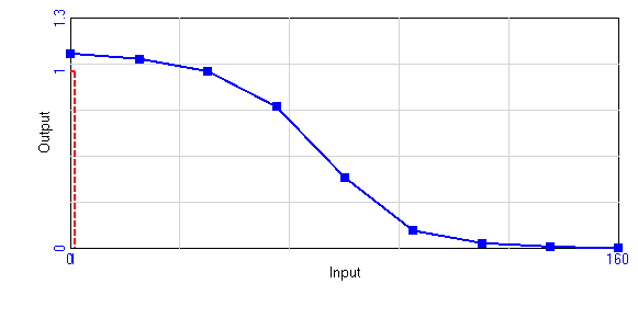
Default	Workweek	L	Table for Effect of Work Pressure on Workweek (Dimensionless) = [(-0.25,0)-(2.25,1.25)],(-0.25,0.75),(0,0.75),(0.25,0.79),(0.5,0.84),(0.75,0.9),(1,1),(1.25,1.09),(1.5,1.17),(1.75,1.23),(2,1.25),(2.25,1.25) Description: High schedule pressure leads to longer hours. Present in 1 view: Backlog Used by: Effect of Work Pressure on Workweek - High schedule pressure leads to overtime; low pressure to a reduction in hours worked.
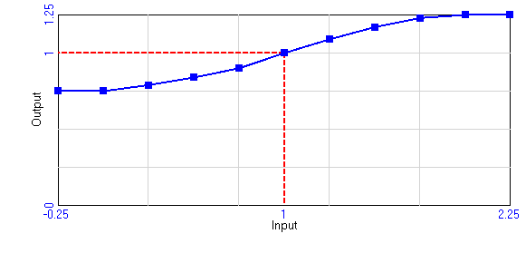
Default	Workweek	A	Workweek (Hours/Week) = Standard WorkweekEffect of Work Pressure on Workweek Description:* The workweek is the standard workweek modified by the effect of schedule pressure on workweek. Present in 2 views: Backlog Responses Used by: Normalized Workweek - Fractional change of the workweek relative to the standard workweek. Potential Completion Rate - The potential completion rate depends on the net available labor force, the workday, and the average time spent on each task. Long Term Workweek - Exponential smoothing of the workweek over the period for the onset of burnout. The 'long term' label refers to the fact that the burnout onset time is much longer than the fatigue onset time. Recent Workweek - Exponential smoothing of the workweek over the period for the onset of fatigue. The 'short term' label refers to the fact that the burnout onset time is much longer than the fatigue onset time.

List of 1 Undocumented Variable

Module	*Group*	Type	Variable (1)
Default	Task Flows	SI,C	Time to Discover Errors (Week)

List of 8 Supplementary Variables

Module	*Group*	Type	Variable (8)
Default	Individual Learning Curve	A	LC (Employees)
Default	Normalized Responses	A	Normalized Completion rate (Dimensionless)
Default	Normalized Responses	A	Normalized Effective Workforce (Dimensionless)
Default	Normalized Responses	A	Normalized Standard Time per Task (Dimensionless)
Default	Normalized Responses	A	Normalized Time per Task (Dimensionless)
Default	Normalized Responses	A	Normalized Workweek (Dimensionless)
Default	Workforce	A	Experienced fraction to training (Dimensionless)
Default	Workforce	A	Rookie fraction (Dimensionless)

Formulation Complexity Summary (Violations of Richardson's Rule)

Module	Group	Type	Variable	Complexity Score
Default	Workforce	S	Experienced Employees (Employees)	4
Default	Workforce	F,A	Experienced Quit Rate (Employees/Week)	4
Default	Time per Task	A	Adjustment Time for Standard Time Per Task (Week)	4
Default	Market Response	F,A	Net Change to Customer Base (Customers/Week)	4
Default	Workforce	F,A	Rookie Quit Rate (Employees/Week)	4
Default	Task Flows	A	Effect of Delivery Delay on Balking (Dimensionless)	4
Default	Task Flows	F,A	Balking Rate (Tasks/Week)	4
Default	Workforce Planning	SM	Desired Workforce (Employees)	4
Default	Workforce Planning	I	Base Budget ($/Week)	4
Default	Workforce Planning	A	Budget ($/Week)	4
Default	Task Flows	S	Service Backlog (Tasks)	5
Default	Workforce	S	Rookie Employees (Employees)	5
Default	Market Response	SM	Service Attractiveness (Dimensionless)	5
Default	Workforce	F,A	Rookie Hire Rate (Employees/Week)	6
Default	Test Generator for Arrivals	A	Input (Dimensionless)	12
Default	Test Generator for Absenteeism	A	Input 0 (Dimensionless)	12

List of 32 Equations with Embedded Data

Module	*Group*	Type	Variable (32)
Default	Market Response	A	Effect of Balking on Attractiveness (Dimensionless)
Default	Market Response	A	Effect of Errors on Attractiveness (Dimensionless)
Default	Test Generator for Absenteeism	A	Absenteeism (Dimensionless)
Default	Test Generator for Absenteeism	A	Input 0 (Dimensionless)
Default	Test Generator for Absenteeism	S	Pink Noise 0 (Dimensionless)
Default	Test Generator for Absenteeism	A	White Noise 0 (Dimensionless)
Default	Individual Learning Curve	S	LC E (Employees)
Default	Individual Learning Curve	S	LC R (Employees)
Default	Normalized Responses	A	Normalized Time per Task (Dimensionless)
Default	Normalized Responses	A	Normalized Workweek (Dimensionless)
Default	Normalized Responses	A	Normalized Standard Time per Task (Dimensionless)
Default	Normalized Responses	A	Normalized Effective Workforce (Dimensionless)
Default	Normalized Responses	A	Normalized Completion rate (Dimensionless)
Default	Service Quality	A	Probability of Error Generation (Dimensionless)
Default	Service Quality	A	Effect of Time per Order on Probability of Error Free (Dimensionless)
Default	Task Flows	SI,F,A	Error Generation Rate (Tasks/Week)
Default	Task Flows	F,A	Balking Rate (Tasks/Week)
Default	Task Flows	A	Effect of Delivery Delay on Balking (Dimensionless)
Default	Task Flows	SI,F,A	Task Arrival Rate (Tasks/Week)
Default	Time per Task	A	Effect of Work Pressure on Time per Task (Dimensionless)
Default	Test Generator for Arrivals	A	Input (Dimensionless)
Default	Test Generator for Arrivals	S	Pink Noise (Dimensionless)
Default	Test Generator for Arrivals	A	White Noise (Dimensionless)
Default	Workweek	A	Effect of Work Pressure on Workweek (Dimensionless)
Default	Workforce	F,A	Rookie Hire Rate (Employees/Week)
Default	Workforce	A	Effective Experienced employees (Employees)
Default	Workforce	S	Experienced Employees (Employees)
Default	Workforce	A	Experienced fraction to training (Dimensionless)
Default	Workforce	SI,A	Steady State Rookie Fraction (Dimensionless)
Default	Workforce Planning	A	Authorized Workforce (Employees)
Default	Workforce Planning	SM	Desired Workforce (Employees)
Default	Workforce Planning	A	Budget ($/Week)

List of 3 Unused Variables

Module	*Group*	Type	Variable (3)
Default	Test Generator for Absenteeism	A	Absenteeism (Dimensionless)
Default	Test Generator for Absenteeism	C	Noise Seed 0 (Dimensionless)
Default	Test Generator for Arrivals	C	Noise Seed (Dimensionless)

List of 8 Views and Their 181 Variables*

	Workforce	Effective, Desired and Authorized Workforce	Backlog	Standard Time per Task	Service Quailty	Task Arrivals and Absenteeism	Responses	Market Response
Total:	41	34	45	7	17	49	14	26	:Total
Absenteeism (in 1 view)						X			Absenteeism (in 1 view)
Adjustment Time for Standard Time Per Task (in 1 view)				X					Adjustment Time for Standard Time Per Task (in 1 view)
Affordable Workforce (in 1 view)		X							Affordable Workforce (in 1 view)
Assimilation Rate (in 1 view)	X								Assimilation Rate (in 1 view)
Assimilation Time (in 2 views)	X	X							Assimilation Time (in 2 views)
Authorized Workforce (in 2 views)	X	X							Authorized Workforce (in 2 views)
Average Productivity (in 2 views)		X			X				Average Productivity (in 2 views)
Balking Rate (in 1 view)			X						Balking Rate (in 1 view)
Base Budget (in 1 view)		X							Base Budget (in 1 view)
Base Customer Growth Rate (in 1 view)								X	Base Customer Growth Rate (in 1 view)
Base Task Arrival Rate (in 1 view)								X	Base Task Arrival Rate (in 1 view)
Budget (in 1 view)		X							Budget (in 1 view)
Burnout Onset Time (in 1 view)			X						Burnout Onset Time (in 1 view)
Capacity Slack Fraction (in 1 view)		X							Capacity Slack Fraction (in 1 view)
Capacity Switch (in 1 view)	X								Capacity Switch (in 1 view)
Change in Pink Noise (in 1 view)						X			Change in Pink Noise (in 1 view)
Change in Pink Noise 0 (in 1 view)						X			Change in Pink Noise 0 (in 1 view)
Change in Standard Time per Task (in 2 views)			X	X					Change in Standard Time per Task (in 2 views)
Cost per Employee (in 1 view)		X							Cost per Employee (in 1 view)
Customer Base (in 2 views)		X						X	Customer Base (in 2 views)
Customer Expected Time Per Task (in 1 view)					X				Customer Expected Time Per Task (in 1 view)
Cutting Corners Switch (in 1 view)			X						Cutting Corners Switch (in 1 view)
Delivered Quality (in 3 views)	X				X			X	Delivered Quality (in 3 views)
Delivery Delay (in 2 views)			X					X	Delivery Delay (in 2 views)
Desired Completion Rate (in 1 view)			X						Desired Completion Rate (in 1 view)
Desired Hiring Rate (in 1 view)	X								Desired Hiring Rate (in 1 view)
Desired Service Capacity (in 2 views)		X	X						Desired Service Capacity (in 2 views)
Desired Vacancies (in 1 view)	X								Desired Vacancies (in 1 view)
Desired Workforce (in 1 view)		X							Desired Workforce (in 1 view)
Effect of Balking on Attractiveness (in 1 view)								X	Effect of Balking on Attractiveness (in 1 view)
Effect of Burnout on Turnover (in 1 view)	X								Effect of Burnout on Turnover (in 1 view)
Effect of Delivered Quality on Attractiveness (in 1 view)								X	Effect of Delivered Quality on Attractiveness (in 1 view)
Effect of Delivery Delay on Attractiveness (in 1 view)								X	Effect of Delivery Delay on Attractiveness (in 1 view)
Effect of Delivery Delay on Balking (in 2 views)			X					X	Effect of Delivery Delay on Balking (in 2 views)
Effect of Errors on Attractiveness (in 1 view)								X	Effect of Errors on Attractiveness (in 1 view)
Effect of Fatigue on Probability of Error Free (in 1 view)					X				Effect of Fatigue on Probability of Error Free (in 1 view)
Effect of Fatigue on Productivity (in 1 view)			X						Effect of Fatigue on Productivity (in 1 view)
Effect of Inexperience on Probability of Error Free (in 1 view)					X				Effect of Inexperience on Probability of Error Free (in 1 view)
Effect of Quality on Turnover (in 1 view)	X								Effect of Quality on Turnover (in 1 view)
Effect of Time per Order on Probability of Error Free (in 1 view)					X				Effect of Time per Order on Probability of Error Free (in 1 view)
Effect of Work Pressure on Time per Task (in 1 view)			X						Effect of Work Pressure on Time per Task (in 1 view)
Effect of Work Pressure on Workweek (in 1 view)			X						Effect of Work Pressure on Workweek (in 1 view)
Effective Experienced employees (in 1 view)		X							Effective Experienced employees (in 1 view)
Effective Workforce (in 3 views)		X	X				X		Effective Workforce (in 3 views)
Employee Vacancies (in 1 view)	X								Employee Vacancies (in 1 view)
Endogenous Task Arrival Rate (in 2 views)			X					X	Endogenous Task Arrival Rate (in 2 views)
Error Discovery Rate (in 2 views)			X					X	Error Discovery Rate (in 2 views)
Error Generation Rate (in 1 view)			X						Error Generation Rate (in 1 view)
Exogenous Task Arrival Rate (in 2 views)			X			X			Exogenous Task Arrival Rate (in 2 views)
Experienced Employees (in 2 views)	X	X							Experienced Employees (in 2 views)
Experienced fraction to training (in 1 view)		X							Experienced fraction to training (in 1 view)
Experienced Quit Fraction (in 1 view)	X								Experienced Quit Fraction (in 1 view)
Experienced Quit Rate (in 1 view)	X								Experienced Quit Rate (in 1 view)
Fatigue Onset Time (in 1 view)			X						Fatigue Onset Time (in 1 view)
FINAL TIME (in 0 views)									FINAL TIME (in 0 views)
Financial Switch (in 1 view)		X							Financial Switch (in 1 view)
Fraction of Revenue for Operations (in 1 view)		X							Fraction of Revenue for Operations (in 1 view)
Fraction of time required to train rookies (in 1 view)		X							Fraction of time required to train rookies (in 1 view)
Growth Rate (in 1 view)	X								Growth Rate (in 1 view)
Hiring Rate (in 1 view)	X								Hiring Rate (in 1 view)
Indicated Labor Order Rate (in 1 view)	X								Indicated Labor Order Rate (in 1 view)
Initial Arrival Rate (in 2 views)						X	X		Initial Arrival Rate (in 2 views)
Initial Effective Workforce (in 1 view)							X		Initial Effective Workforce (in 1 view)
Initial employees (in 1 view)	X								Initial employees (in 1 view)
Initial Standard Time per Task (in 4 views)			X	X	X		X		Initial Standard Time per Task (in 4 views)
INITIAL TIME (in 0 views)									INITIAL TIME (in 0 views)
Input (in 2 views)						X		X	Input (in 2 views)
Input 0 (in 1 view)						X			Input 0 (in 1 view)
Labor Order Rate (in 1 view)	X								Labor Order Rate (in 1 view)
LC (in 1 view)		X							LC (in 1 view)
LC AR (in 1 view)		X							LC AR (in 1 view)
LC E (in 1 view)		X							LC E (in 1 view)
LC R (in 1 view)		X							LC R (in 1 view)
Long Term Workweek (in 2 views)	X		X						Long Term Workweek (in 2 views)
Margin for Reserve Capacity (in 1 view)		X							Margin for Reserve Capacity (in 1 view)
Market Feedback Switch (in 1 view)			X						Market Feedback Switch (in 1 view)
Maximum Completion Rate (in 1 view)			X						Maximum Completion Rate (in 1 view)
Minimum Delivery Delay (in 1 view)			X						Minimum Delivery Delay (in 1 view)
Net Change to Customer Base (in 1 view)								X	Net Change to Customer Base (in 1 view)
Noise Correlation Time (in 1 view)						X			Noise Correlation Time (in 1 view)
Noise Correlation Time 0 (in 1 view)						X			Noise Correlation Time 0 (in 1 view)
Noise Seed (in 1 view)						X			Noise Seed (in 1 view)
Noise Seed 0 (in 1 view)						X			Noise Seed 0 (in 1 view)
Noise Standard Deviation (in 1 view)						X			Noise Standard Deviation (in 1 view)
Noise Standard Deviation 0 (in 1 view)						X			Noise Standard Deviation 0 (in 1 view)
Noise Start Time (in 1 view)						X			Noise Start Time (in 1 view)
Noise Start Time 0 (in 1 view)						X			Noise Start Time 0 (in 1 view)
Normal Balking Rate (in 1 view)			X						Normal Balking Rate (in 1 view)
Normalized Completion rate (in 1 view)							X		Normalized Completion rate (in 1 view)
Normalized Effective Workforce (in 1 view)							X		Normalized Effective Workforce (in 1 view)
Normalized Standard Time per Task (in 1 view)							X		Normalized Standard Time per Task (in 1 view)
Normalized Time per Task (in 1 view)							X		Normalized Time per Task (in 1 view)
Normalized Workweek (in 1 view)							X		Normalized Workweek (in 1 view)
Perceived Employee Effectiveness (in 1 view)		X							Perceived Employee Effectiveness (in 1 view)
Pink Noise (in 1 view)						X			Pink Noise (in 1 view)
Pink Noise 0 (in 1 view)						X			Pink Noise 0 (in 1 view)
Potential Completion Rate (in 1 view)			X						Potential Completion Rate (in 1 view)
Probability of Error Generation (in 2 views)			X		X				Probability of Error Generation (in 2 views)
Pulse Duration (in 1 view)						X			Pulse Duration (in 1 view)
Pulse Duration 0 (in 1 view)						X			Pulse Duration 0 (in 1 view)
Pulse Quantity (in 1 view)						X			Pulse Quantity (in 1 view)
Pulse Quantity 0 (in 1 view)						X			Pulse Quantity 0 (in 1 view)
Pulse Time (in 1 view)						X			Pulse Time (in 1 view)
Pulse Time 0 (in 1 view)						X			Pulse Time 0 (in 1 view)
Ramp End Time (in 1 view)						X			Ramp End Time (in 1 view)
Ramp End Time 0 (in 1 view)						X			Ramp End Time 0 (in 1 view)
Ramp Slope (in 1 view)						X			Ramp Slope (in 1 view)
Ramp Slope 0 (in 1 view)						X			Ramp Slope 0 (in 1 view)
Ramp Start Time (in 1 view)						X			Ramp Start Time (in 1 view)
Ramp Start Time 0 (in 1 view)						X			Ramp Start Time 0 (in 1 view)
Recent Workweek (in 2 views)			X		X				Recent Workweek (in 2 views)
Replacement Rate (in 1 view)	X								Replacement Rate (in 1 view)
Revenue (in 1 view)		X							Revenue (in 1 view)
Revenue per Customer (in 1 view)		X							Revenue per Customer (in 1 view)
Rookie Employees (in 2 views)	X	X							Rookie Employees (in 2 views)
Rookie fraction (in 1 view)	X								Rookie fraction (in 1 view)
Rookie Hire Rate (in 1 view)	X								Rookie Hire Rate (in 1 view)
Rookie productivity fraction (in 1 view)		X							Rookie productivity fraction (in 1 view)
Rookie Quit Fraction (in 1 view)	X								Rookie Quit Fraction (in 1 view)
Rookie Quit Rate (in 1 view)	X								Rookie Quit Rate (in 1 view)
SAVEPER (in 0 views)									SAVEPER (in 0 views)
Sensitivity of Attractiveness to Balking (in 1 view)								X	Sensitivity of Attractiveness to Balking (in 1 view)
Sensitivity of Attractiveness to Delivered Quality (in 1 view)								X	Sensitivity of Attractiveness to Delivered Quality (in 1 view)
Sensitivity of Attractiveness to Delivery Delay (in 1 view)								X	Sensitivity of Attractiveness to Delivery Delay (in 1 view)
Sensitivity of Attractiveness to Errors (in 1 view)								X	Sensitivity of Attractiveness to Errors (in 1 view)
Sensitivity of Balking to Delivery Delay (in 1 view)			X						Sensitivity of Balking to Delivery Delay (in 1 view)
Sensitivity of Errors to Time per Task (in 1 view)					X				Sensitivity of Errors to Time per Task (in 1 view)
Service Attractiveness (in 1 view)								X	Service Attractiveness (in 1 view)
Service Backlog (in 1 view)			X						Service Backlog (in 1 view)
Service Capacity (in 2 views)		X	X						Service Capacity (in 2 views)
Sine Amplitude (in 1 view)						X			Sine Amplitude (in 1 view)
Sine Amplitude 0 (in 1 view)						X			Sine Amplitude 0 (in 1 view)
Sine Period (in 1 view)						X			Sine Period (in 1 view)
Sine Period 0 (in 1 view)						X			Sine Period 0 (in 1 view)
Standard Completion Rate (in 2 views)						X		X	Standard Completion Rate (in 2 views)
Standard Time per Task (in 3 views)			X	X			X		Standard Time per Task (in 3 views)
Standard Workweek (in 4 views)	X		X		X		X		Standard Workweek (in 4 views)
Steady State Rookie Fraction (in 1 view)	X								Steady State Rookie Fraction (in 1 view)
Step Height (in 1 view)						X			Step Height (in 1 view)
Step Height 0 (in 1 view)						X			Step Height 0 (in 1 view)
Step test switch (in 1 view)	X								Step test switch (in 1 view)
Step Time (in 1 view)						X			Step Time (in 1 view)
Step Time 0 (in 1 view)						X			Step Time 0 (in 1 view)
Table for Delivered Quality (in 1 view)					X				Table for Delivered Quality (in 1 view)
Table for Effect of Burnout on Turnover (in 1 view)	X								Table for Effect of Burnout on Turnover (in 1 view)
Table for Effect of Fatigue on PEF (in 1 view)					X				Table for Effect of Fatigue on PEF (in 1 view)
Table for Effect of Fatigue on Productivity (in 1 view)			X						Table for Effect of Fatigue on Productivity (in 1 view)
Table for Effect of Inexperience on PEF (in 1 view)					X				Table for Effect of Inexperience on PEF (in 1 view)
Table for Effect of Quality on Turnover (in 1 view)	X								Table for Effect of Quality on Turnover (in 1 view)
Table for Effect of Work Pressure on Time per Task (in 1 view)			X						Table for Effect of Work Pressure on Time per Task (in 1 view)
Table for Effect of Work Pressure on Workweek (in 1 view)			X						Table for Effect of Work Pressure on Workweek (in 1 view)
Target Delivered Quality (in 1 view)								X	Target Delivered Quality (in 1 view)
Target Delivery Delay (in 2 views)			X					X	Target Delivery Delay (in 2 views)
Task Arrival Rate (in 1 view)			X						Task Arrival Rate (in 1 view)
Task Completion Rate (in 3 views)			X				X	X	Task Completion Rate (in 3 views)
Task Request per Customer (in 1 view)								X	Task Request per Customer (in 1 view)
Threshold Delivery Delay for Balking (in 1 view)			X						Threshold Delivery Delay for Balking (in 1 view)
Time (in 1 view)						X			Time (in 1 view)
Time for Customer Base to Change (in 1 view)								X	Time for Customer Base to Change (in 1 view)
Time per Task (in 4 views)			X	X	X		X		Time per Task (in 4 views)
TIME STEP (in 1 view)						X			TIME STEP (in 1 view)
Time to Adjust Affordable Workforce (in 1 view)		X							Time to Adjust Affordable Workforce (in 1 view)
Time to Adjust Desired Workforce (in 1 view)		X							Time to Adjust Desired Workforce (in 1 view)
Time to Adjust Workforce (in 1 view)	X								Time to Adjust Workforce (in 1 view)
Time to Cancel Vacancies (in 1 view)	X								Time to Cancel Vacancies (in 1 view)
Time to Decrease Standard Time per Task (in 1 view)				X					Time to Decrease Standard Time per Task (in 1 view)
Time to Discover Errors (in 1 view)			X						Time to Discover Errors (in 1 view)
Time to Hire (in 1 view)	X								Time to Hire (in 1 view)
Time to Increase Standard Time per Task (in 1 view)				X					Time to Increase Standard Time per Task (in 1 view)
Time to Perceive Productivity (in 1 view)		X							Time to Perceive Productivity (in 1 view)
Time to React to Service Attractiveness (in 1 view)								X	Time to React to Service Attractiveness (in 1 view)
Total Employees (in 2 views)	X	X							Total Employees (in 2 views)
Total Quit Rate (in 1 view)	X								Total Quit Rate (in 1 view)
Undiscovered Errors (in 1 view)			X						Undiscovered Errors (in 1 view)
Vacancy Adjustment Rate (in 1 view)	X								Vacancy Adjustment Rate (in 1 view)
White Noise (in 1 view)						X			White Noise (in 1 view)
White Noise 0 (in 1 view)						X			White Noise 0 (in 1 view)
Work Pressure (in 1 view)			X						Work Pressure (in 1 view)
Workforce Adjustment Rate (in 1 view)	X								Workforce Adjustment Rate (in 1 view)
Workweek (in 2 views)			X				X		Workweek (in 2 views)
Workweek Switch (in 1 view)			X						Workweek Switch (in 1 view)
Total:	41	34	45	7	17	49	14	26	:Total
	Workforce	Effective, Desired and Authorized Workforce	Backlog	Standard Time per Task	Service Quailty	Task Arrivals and Absenteeism	Responses	Market Response

Warnings

Model's VPM file does not exist: images unavailable.

Variables in this model have not been completely grouped.

Source file: Handbook Model.mdl (7/1/09 - 2:01 PM)
Created on 8/2/10 - 9:19 AM
SDM-Doc Tool Beta Version 4.1.30
Decision and Information Sciences Division
Argonne National Laboratory